

SOURCE:https://miro.medium.com/max/1075/1*10t9S7xvWE5Z3NEZrmHG2w.jpeg
When teaching machine learning algorithms, the bias-variance trade-off is a problem we both face. Bagging is a powerful tool for the ensemble learning that helps to minimize variation and avoid overfitting by extension. Ensemble approaches boost model consistency by using a group (or “ensemble”) of models that when combined, when used separately, outperform individual models.
In this post, we’ll look at the inner-workings of bagging, its implementations, and use the scikit-learn library to apply the bagging algorithm.
Why Use Ensemble learning?
What we call a strong learner will result from combining many weak models.
To integrate different models, we can use ensemble approaches in two ways: either using a single base learning algorithm that stays the same for all models (a homogeneous ensemble model), or using several base learning algorithms that vary with each model (a heterogeneous ensemble model).
Generally speaking, for decision trees, ensemble learning is use because it is a consistent way to accomplish regularization. In general, as the number of levels in a decision tree grows, the model becomes vulnerable to high variance and can overfit (resulting in high error on test data). In order to enforce regularization and avoid overfitting, we use ensemble procedures with generic laws (vs. extremely detailed rules).
Advantages of This learning
Using a real-life example, let’s consider the benefits of ensemble learning. Consider a situation where you want to predict whether real or spam is an incoming email. By looking at several characteristics separately, you want to predict the type (genuine/spam): if the sender is on your contact list or not, whether the substance of the message relates to money theft, if the vocabulary used is clean and understandable, etc.
Even on the other hand, you would like to jointly estimate the class of the email using all these attributes. As a no-brainer, the following choice fits best when we jointly consider all the attributes, while we independently consider each attribute in the former one. The group ensures the robustness and reliability of the outcome as it generates after a detailed analysis.
This sets forth the strengths of ensemble learning:
- Predictions are Reliable
- Ensures the model’s stability/ robustness.
In most implementations, Ensemble Learning is also the most preferred choice to take advantage of these advantages. Let’s explain a common Ensemble Learning strategy, Bagging, in the next section.
Bagging
The accumulation of several iterations of a predicted model is bagging, also refer as bootstrap aggregating.
Each model is independently train, using an averaging method, and combine. The primary goal of bagging is to produce less variation individually than every model has. Let’s first grasp the word bootstrapping, in order to understand bagging.
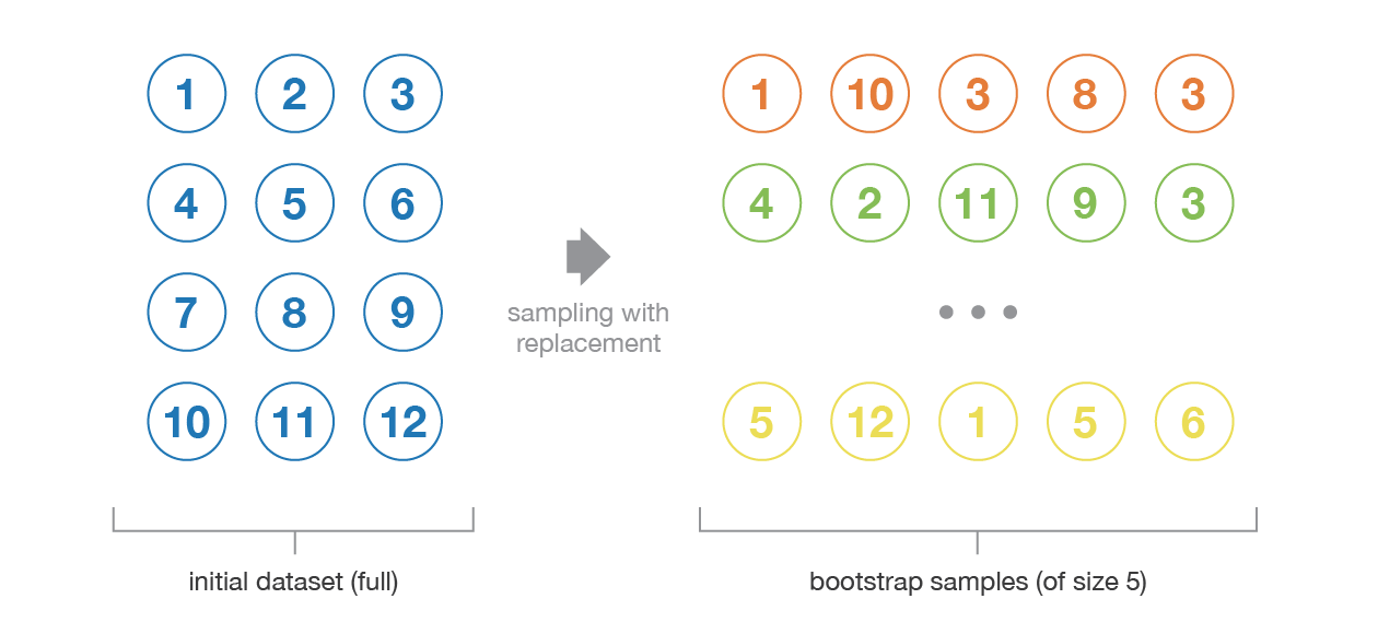
Bootstrapping
The method of producing bootstrapped samples from the given dataset is bootstrapping. The samples are formulate by drawing randomly with substitution data points.
The resampled data incorporates numerous features that are in the original data as a whole. It draws the distribution in the data points, which therefore appears to remain distinct from each other, i.e. the distribution of data must remain unchanged while preserving the bootstrapped samples’ dissimilarity. In exchange, this assists in the development of stable models.
SOURCE: https://towardsdatascience.com/ensemble-methods-bagging-boosting-and-stacking-c9214a10a205
Bootstrapping tends to prevent the topic of overfitting as well. The model becomes resilient to producing errors as various sets of training data are in use in the model, and hence works well with the test data, thus reducing the uncertainty by retaining its large footprint in the test data. Checking with multiple combinations does not skew the paradigm toward a wrong answer.
Today, as we attempt to create fully independent models, massive quantities of data are require. Bootstrapping is therefore the alternative that we decide for by using the dataset’s approximate properties under consideration.
It all began in the year 1994 when this algorithm, then known as “Bagging Predictors,” was propose by Leo Breiman. The bootstrapped samples are produce first in Bagging. Then each sample adds up to either a regression or classification algorithm.
Finally, an estimate is taken of all the outcomes expected by the individual learners in the case of regression. Either the most voted class is approved for designation (hard-voting), or the highest average of all the class probabilities is taken as the performance (soft-voting). This is where it fits into the image of aggregation.
Bagging is defined mathematically by the following formula:
fbag=f1(X)+f2(X)+f3(X)+……….+ fb(X)
Where fbag represents the prediction which is bagged and RHS is the learners which are individual.
When the learners are erratic and appear to overfit, bagging works extremely well, i.e. subtle differences in the training data contribute to large changes in the planned performance. By aggregating the individual learners composed of various statistical properties, such as various standard deviations, means, etc it effectively decreases the variance. For high variance models, such as Decision Trees, it fits well. It doesn’t really affect the learning process as used in low variance models such as linear regression. The number of base learners (trees) to pick depends on the dataset’s characteristics. It does not lead to overfitting by using too many trees, but can use a lot of processing resources.
In order to hold an eye on unnecessary processing power, bagging can be performed in parallel. This is a positive asset that comes with it, and is also a multiplier in a number of ways to improve the algorithm’s use.
BAGGING AND ITS USES
In a wide range of applications, bagging technology is utilize. One key benefit is that by producing additional data, it eliminates the uncertainty of estimation by adding multiple variations and repetitions (replacements in the bootstrapped samples) to the training data. Any applications where the bagging algorithm is commonly use are below:
- Banking Sector
- Predictions in Medical Evidence
- High-dimensional details
- Mapping of Ground Cover
- Detection of Fraud
- Intrusion Prevention Mechanisms for Networks
- Health areas, such as prosthetics, neuroscience, etc.
PROS AND CONS OF BAGGING
Let’s first explore the benefits. Bagging is an algorithm which is fully data-specific. Model overfitting is minimize by the bagging process. On high-dimensional data, it also performs well. In comparison, the missing values in the dataset do not impact the algorithm’s output.
That being said one of the drawbacks it has is to give its final prediction based on the mean predictions of the subset trees, instead of producing the exact values for the model of classification or regression.
ALGORITHM
Let’s look at the walk through the process that goes into the Bagging algorithm implementation. The first step in the flow of the bagging process involves bootstrapping, where the data is broke into random samples.
Then, match each of these samples with another algorithm (e.g. Decision Trees). In parallel, preparation occurs.
Take an average of all the outputs, or compute the sum output in total.
The Hyperparameters encoding
For bagging, Scikit-learn has two classes, one for regression (sklearn, ensemble, BaggingRegressor) and one for classification (sklearn, ensemble, BaggingClassifier). Both embrace different parameters that in conjunction with the given data, will increase the model’s speed and accuracy. There are some of these that include:
Base estimator: the algorithm to be in use on all the dataset’s random subsets. A decision tree is the default attribute.
N-estimators: The number of the ensemble’s foundation estimators. 10 is the default rating.
Random state: The seed used for the generator of random states. None is the default value.
N jobs: With both the fit and expect approaches, the number of jobs to be run in parallel. None is the default value.
Cross-Validation K-Folds is used. To generate train and test data, it yields the train/test indices. The number of folds is calculated by the parameter n splits (default value is 3).
Instead of breaking the data into training and test sets, we use K Folds along with the cross val score to approximate the accuracy. By cross-validation, this approach assesses the score.
Here’s a look at the parameters specified in cross_val_score:
Estimator: The model for the data to match.
X: Data input to suit.
Y: The goal values that the precision is predicted against.
CV: Specifies the strategy of cross-validation splitting. 3 is the default value.
IMPLEMENTATION
The below algorithm is a general algorithm. Depending upon the data set it further has to be manipulated.
Step 1: Modules to Import
We start by importing the required packages that are needed to create our model of bagging. For the loading of our dataset, we use the Pandas data processing library. Any data can be imported from any site.
Next, let’s use the BaggingClassifierfrom the package sklearn.ensemble, and the DecisionTreeClassifier from the package sklearn.tree.
Step 2: The Dataset is load
The dataset can be downloaded from any source. Then in a variable called url, we store the relation. In a list named names, we name all the groups in the dataset. To load the dataset, we use the read_csv method from Pandas and then set the class names to our vector using the ‘names’ parameter, often called names. Next, using the slicing operation, we load the functions and target variables and assign them to variables X and Y, respectively.
Step 3: Classifier loading
In this step, we set the seed value for all the random states, such that once the seed value is exhaust up, the random values will remain the same. We now identify the KFold model in which we set the parameter n_splits to 10, and the parameter random_state to the value of the seed. Here with the Classification and Regression Trees algorithm, we can construct the bagging algorithm.
Step 4: Learning
Using the BaggingClassifier, we train the model in the last step by declaring the parameters with the values specified in the previous step.
By using the parameters, Bagging model, X, Y, and the kfold model, we then verify the model’s results.
It will be spot that Bagging has more efficiency and is better compare to the Decision Tree algorithm. Bagging increases the model’s accuracy and precision by reducing the uncertainty at the expense of being computationally costly. However in modeling a solid architecture, it is also a leading light. The perfection of a model does not only attribute its performance to the algorithm use but also if the algorithm use is the correct one!
Written By: Aryaman Dubey
Reviewed By: Krishna Heroor
If you are Interested In Machine Learning You Can Check Machine Learning Internship Program
Also Check Other Technical And Non Technical Internship Programs