
Getting familiar with Clustering
Many items about us can be classified as this and that,” or we have groupings that may be binary or categories that can be more than two, such as a form of cell phone or genre of book that you may like to buy, to be less abstract and more precise. Predefine classes and the process forecasting that is an important process in the Data Science stack refer Classification are always clear the choices or how the technological lingo wants to put it.
But what if we put a search into play where initially we do not have pre-defined choices, rather we derive those choices! Choices that are based on hidden trends, fundamental correlations between the constituent variables, knowledge characteristics, etc. This approach is refers to as Machine Learning Clustering or Cluster Analysis, where we group the data into an several number of groups and later use the knowledge for further business processes.
the mechanism by which we build classes in a data, such as clients, goods, workers, text records, is in mL clustering. in such a way that objects falling into one category exhibit several related properties with each other and are distinct from objects falling in the other groups that were generate during the process.
Clustering algorithms take the data and shape these classes using some kind of similarity metrics, which can later be in use in various business processes such as data extraction, pattern recognition, image analysis, data compression, bioinformatics, etc. As mentioned above a distance-based similarity metric plays a crucial role in the clustering decision in the Machine Learning framework for Clustering.
Methods:
As already mentioned at a point earlier, we need to accomplish two key targets for a good grouping: one a resemblance between one data point with another and two, a differentiation between such identical data points with others that definitely vary heuristically from those points. With our capacity to scale massive datasets, the cornerstone of those divisions starts and it is a big starting point for us.
If we are through it we face with a challenge that our information includes various kinds of characteristics, categorical, continuous results, etc., and we should be able to deal with them. Now, we know that these days, our data is not confine in terms of dimensions, we have multi-dimensional data. This barrier can also be effectively reach by the clustering algorithm.
The clusters we need should not only be able to discriminate between data points, but they should also be inclusive. A separation variable definitely helps a lot, but the shape of the cluster also restricts to being a geometric shape and several relevant data points are omit. This thing needs to be care of .
We note in our development that our data is extremely noisy” in nature. There have been several unnecessary features in the data that make it a very Herculean task to establish some similarity between the data points, contributing to the formation of inappropriate classes.

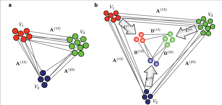
SOURCE: https://ars.els-cdn.com/content/image/1-s2.0-S0925231217311815-gr1.jpg
Types of clustering
1. Hierarchical clustering
Hierarchical Clustering is a clustering process in unsupervised machine learning where it starts from a predefined top-to-bottom cluster hierarchy. It then continues to do a decomposition based on this hierarchy of the data objects, thereby obtaining the clusters. Based on the course of development, this process assumes two methods, i.e. whether it is the top-down or bottom-up cluster formation flow. Both are the Agglomerative Approach and the Divisive Approach.

2. Divisive Approach:-
This hierarchical clustering strategy approaches a top-down approach where we assume that all data points belong to a single large cluster and attempt to break the data into smaller classes based on a termination logic or a point after which no further split of data points can take place. This termination logic may be based on the minimum total of error squares inside a cluster, or the GINI coefficient inside a cluster may be the metric for categorical results.
Therefore the data that was once cluster as a single large cluster is iteratively separates into “n” numbers of smaller clusters to which the data points now belong.
It must be consider into account that when separating the clusters, this algorithm is strongly “rigid,”. thus, meaning that if a clustering completes within a loop, there is no way that the task can be reversed.
Function used for Divisive Analysis
In R, the diana() function is in use from the cluster module (cluster::diana)
3. Agglomerative Approach
In comparison to Divisive, agglomerative is just the reverse, where all “N” data points are assumes to be a single component of “N” clusters of which the data is constitute. We merge these various “N” clusters iteratively into smaller clusters, let’s assume “k” clusters, and then allocate the data points accordingly to each of these clusters. This technique is a bottom-up one and in merging the clusters, it also uses a termination logic.
This logic can be a criterion upon a number (no more clusters past this point) or a criterion for distance (clusters should not be too far apart to be merge) or a criterion for variance (increase in the variance of the cluster being merge should not exceed a threshold, Ward Method).
AlGORITHM :(AGGLOMERATIVE NESTING or AGNES)
AGNES begins by realising that each data point has its own cluster, i.e., if there are n data rows, the algorithm initially starts with n clusters. Then, iteratively, clusters that are most similar are now group to form a bigger cluster, again based on the distances as calculate in DIANA. The iterations are carry out until one big cluster that comprises all the data points is left with us.
Implementation:
In R, we use the agnes() function from the cluster package (cluster::agnes()) or from the native stats package, the built-in hclust() function. The implementation can be find in the scikit-learn package inside the cluster module via the Agglomerative Clustering feature in python (sklearn.cluster.AgglomerativeClustering).
Advantages:
- No prior information requires about the number of clusters, although a threshold for divisions needs to be establish by the user.
- Easy to incorporate through multiple data formats and proven to produce robust outcomes for data generated from multiple sources. Therefore, it has a wide field of use.
Disadvantages:
- The division of the cluster (DIANA) or combination (AGNES) is very strict and can not be incomplete and reassign in future iterations or re-runs once perform.
- It has a high time complexity with all the n data-points in the order
O(n2 logn), so it can not be in use for larger datasets.
3. Unable to cope with outliers and noise
Areas of application:
1. Widely used to study evolutionary history and the relationships between biological organisms in DNA sequencing (Phylogenetics).
2. By clustering the news item corpus, assigning the tokens or terms into these clusters and marking out dubious and sensationalised words to get potential false words, detecting fake news.
There are many more methods of clustering. Let us look at Fuzzy Clustering briefly.
FUZZY CLUSTERING
The basic clustering principle revolves around assigning data points to clusters that are mutually exclusive, meaning that a data point only exists within a cluster and does not belong to more than one cluster. Fuzzy clustering approaches modify this model by assigning a data point with a quantified degree of ownership metric to several clusters. The data points at the middle of the cluster can also belong to a cluster that is larger than the points at the edge of the cluster. The probability of an element belonging to a given cluster is determined by a coefficient of membership that ranges from 0 to 1.
For datasets where the variables have a high degree of overlap, fuzzy clustering can be used. It is a widely common image segmentation algorithm, especially in bioinformatics, where the detection of overlapping gene codes makes it difficult for generic clustering algorithms to discriminate between the pixels of the image and fail to perform proper clustering.
ALGORITHM: FUZZY C MEANS (FANNY)
SOURCE: https://pythonhosted.org/scikit-fuzzy/_images/plot_cmeans_1.png
The fuzzy cluster assignment technique in clustering follows this algorithm. The operation of the FCM Algorithm is almost identical to the distance-based cluster assignment of k-means, but the key distinction that a data point can be placed into more than one cluster according to this algorithm. As seen below, this degree of belonging can be easily seen in this algorithm’s cost function:
J=1KxiCjuij m(xi-uj)2
Uij is the degree to which data xi belongs to the cjj cluster.
μj is the centre of the unit of the j cluster,
The fuzzifier is m.
So, much like the k-means algorithm, the number of clusters k is first specified and then the degree of belonging to the cluster is given. The algorithm must then be replicated before the max iterations are achieved, which can again be tuned according to the specifications.
R Implementation
In R, FCM can be introduced from the cluster bundle (cluster::fanny) using fanny() and in Python, fuzzy clustering can be achieved from the skfuzzy module using the cmeans() function. (skfuzzy.cmeans) which can be modified using the prediction function (skfuzzy.cmeans predict) to be applied to new results.
Advantages:
- FCM works well for strongly clustered and overlapping data, where no definitive findings can be provided by k-means.
- It is an unsupervised algorithm and has a higher convergence rate than other algorithms based on partitioning.
Disadvantages:
- Before the start of the algorithm, we must determine the number of ‘k’ clusters.
- Although convergence is still assured, the mechanism is very slow and larger data can not be used for this.
Application regions
- Used extensively in medical image segmentation, particularly the images produced by an MRI.
- Description of the industry and segmentation.
There are various types of clustering like centroid based, Density based, Distribution based etc. and associated algorithms of each type of clustering. Depending on the situation, the type of clustering method is chosen and applied.
Written By: Aryaman Dubey
Reviewed By: Krishna Heroor
If you are Interested In Machine Learning You Can Check Machine Learning Internship Program
Also Check Other Technical And Non Technical Internship Programs