
I think you have got the idea by seeing the Decision Tree itself.
- What is a Decision Tree?
- Why do we use Decision Trees?
- How does a Decision Tree work?
So yes, the above are the basic questions that raise when we think about
Decision Tree Algorithm. You will find all the answers in this blog. Let’s get started.
What is a Decision Tree?
A decision tree is a decision support tool that uses a tree-like model of decisions and their possible consequences, including chance event outcomes, resource costs, and utility. It is one way to display an algorithm that only contains conditional control statements.
Example:
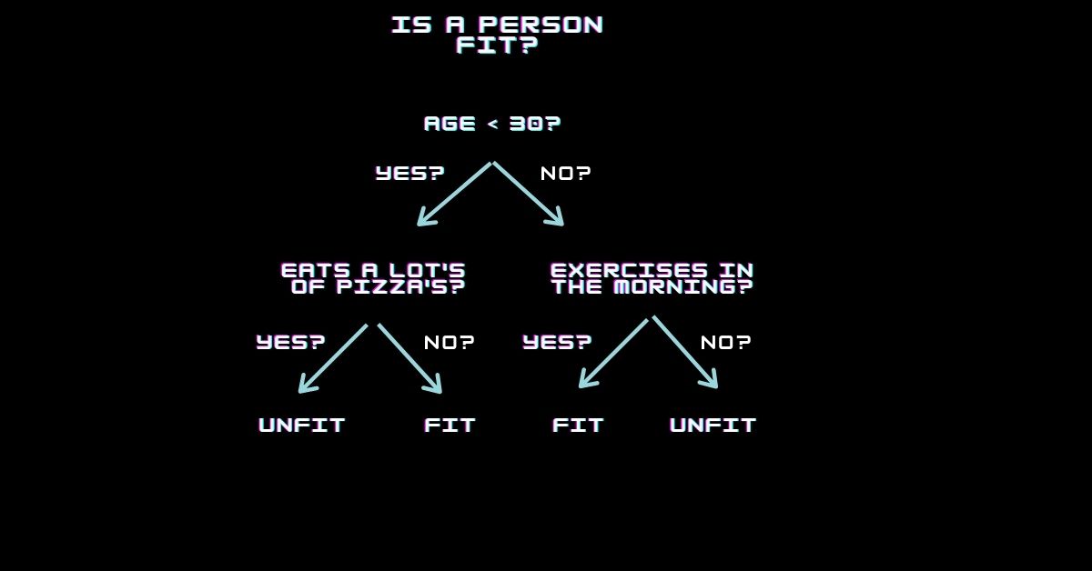
So in the above example figure, I have derived an example for making a decision statement using Decision Tree structure. So, the Decision Tree Algorithm will predict whether the person is Fit or Unfit using some statistics. This is just a sample example to show how a Decision Tree classifies data.
Decision Tree is of Two Types:
1. Regression Tree
Mean of response variable became a prediction for that class.
For continuous quantitative target variables.
Eg. Predicting rainfall, predicting revenue, predicting marks etc.
2. Classification Tree
We use mode (most frequent category in that region will be the prediction)
For discrete categorical target variables.
Eg. Predicting High or Low, Win or Loss, Healthy or Unhealthy etc.
Splitting the nodes in Regression Tree:
We are going to know more about the Decision Tree, how it arranges the data and predicts the output in the Regression Tree.

Now, we have taken another example to create a decision tree where we took a dataset for predicting the score using Midterm marks also based on the hours they studied in Midterm exam using these two columns we will predict the final score of a student We have divided the data using the mean value of the Midterm column. In the above figure we can see that it constructed a Decision tree. This type of split is done in the Regression Tree.
TERMINOLOGIES:
Root Node: The Root node represents the entire data we are using, and it further divides into two or more heterogeneous datasets.
Splitting: The process of dividing the node into two or more sub-nodes based on the condition we applied.
Decision Node: Based on the condition the Decision node further divides into two or more sub-nodes
Subtree: A subsection of the entire tree is called the subtree.
Leaf/Terminal Node: The node which cannot further divide into sub-node is called leaf/terminal node.
The Decision Tree in the above picture is divided using the Mean value of the Midterm column. We have splitted the data using some conditions as you can see students who studied hours<10 are placed on the left and students who studied more than 10 hrs are moved to the right subtree.
How a Decision Tree works?
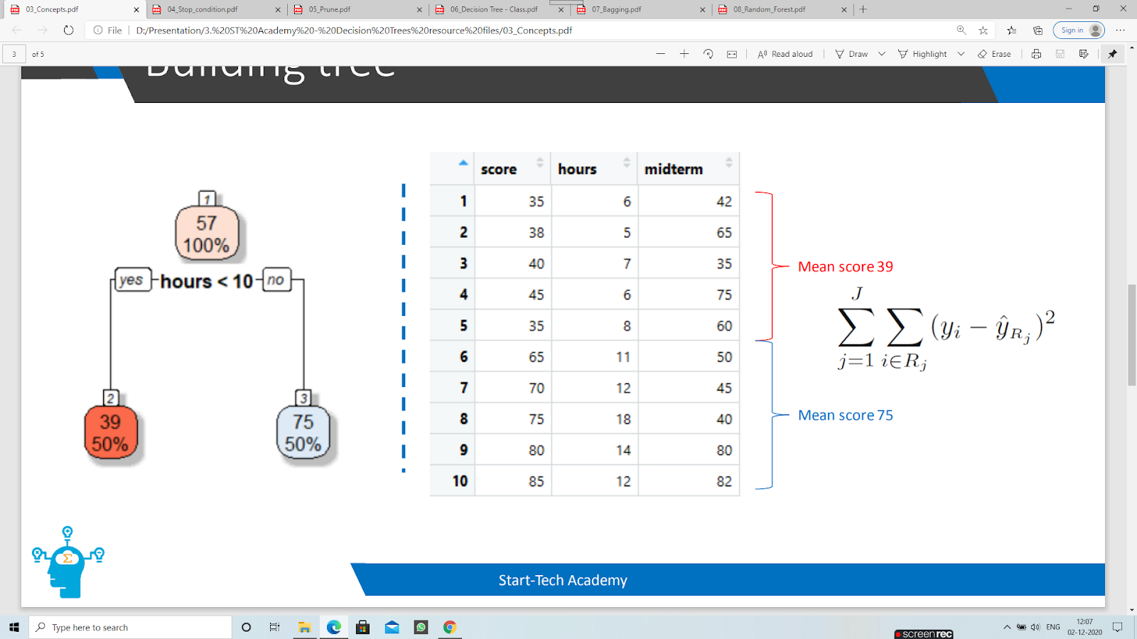
As earlier I said that the decision tree is divided based on the mean value of the Midterm score. Calculate the mean of the Midterm column you will get 57.4
ground that value to 57. Now who studied more than10 hours will score above 57 marks in the final exam and less than 10 will score below 57. Using this data we will predict the final score. We use RSS for Regression Tree.

1. We divide the predictor space—that is, the set of possible values for X1,X2, . . .,Xp—into J distinct and non-overlapping regions, R1,R2, . . . , RJ .
2. For every observation that falls into the region Rj, we make the same prediction, which is simply the mean of the response values for the training observations in Rj .
Goal is to minimize RSS

Approach:
- Top-down, greedy approach that is known as recursive binary splitting.
- Top-down because it begins at the top of the tree and then successively splits the predictor space.
- Each split is indicated via two new branches further down on the tree.
- It is greedy because at each step of the tree-building process, the best split is made at that particular step, rather than looking ahead and picking a split that will lead to a better tree in some future step.
Steps:
- Consider all predictors and all possible cut point values.
- Calculates RSS for each possibility.
- Selects the one with least RSS.
- Continues till stopping criteria is reached.
Stopping Criteria:
- Minimum Observations at internal node Minimum numbers of observations required for further split.
- Minimum Observations at leaf node Minimum number of observations needed at each node after splitting.
- Maximum depth Maximum layers of tree possible.
This is how we split the nodes in the Regression Tree and build the tree until we reach the stopping criteria.
Pruning:
Pruning is a technique used to control the growth of a decision tree because a fully grown tree is overfit for a model.

In pruning, you trim off the branches of the tree, i.e., remove the decision nodes starting from the leaf node such that the overall accuracy is not disturbed. This is done by segregating the actual training set into two sets: training data set, D and validation data set, V. Prepare the decision tree using the segregated training data set, D. Then continue trimming the tree accordingly to optimize the accuracy of the validation data set, V.
In the above diagram the Criminal record attribute in the Right-Hand-Side of the tree is pruned, as it has no importance in the tree, hence removing overfitting.
Ensemble Methods:
The ensemble methods are used because when we fit our model using classification trees we get a high variance. So we choose ensemble methods for fitting the model. We will discuss these ensemble techniques later.
Problem with normal decision tree = High Variance
Splitting the nodes in Classification Tree:
Now let’s see how the Classification Tree splits the attributes using the above stated measures.
Regression RSS is used to decide the split.
In Classification we can use.
- Classification error rate
- Gini Index
- Cross Entropy
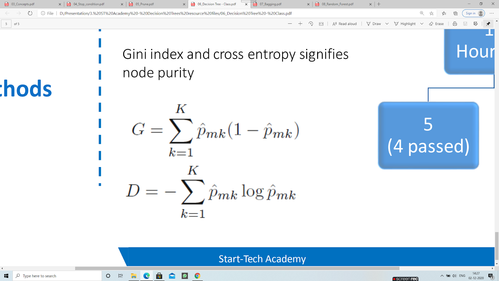
Gini index and cross entropy signifies node purity.

I’m using the below table data to calculate the entropy value.
Here the decision column is the target column we are going to use for splitting the nodes for a Classification tree.
Entropy:
Entropy is a measure of the randomness in the information being processed. The higher the entropy, the harder it is to draw any conclusions from that information. Flipping a coin is an example of an action that provides information that is random.
Entropy Formula:
We have taken decision values as it is a categorical variable there are two types “YES” and “NO” totally 14 values, 9(YES) category values and 5(NO)category values we will divide with 14 and apply log function on it.
Entropy(Decision) = –[p(9/14).log2p(9/14)+p(5/14).log2p(5/14)]
=-[(0.642)(-0.639)+(0.357)(-1.486)]
= -[-0.410+0.530] = -[-0.94] = 0.940
Gini: You can understand the Gini index as a cost function used to evaluate splits in the dataset. It is calculated by subtracting the sum of the squared probabilities of each class from one. It favors larger partitions and is easy to implement whereas information gain favors smaller partitions with distinct values.

Higher the value of Gini index higher the homogeneity.
Gini Formula:
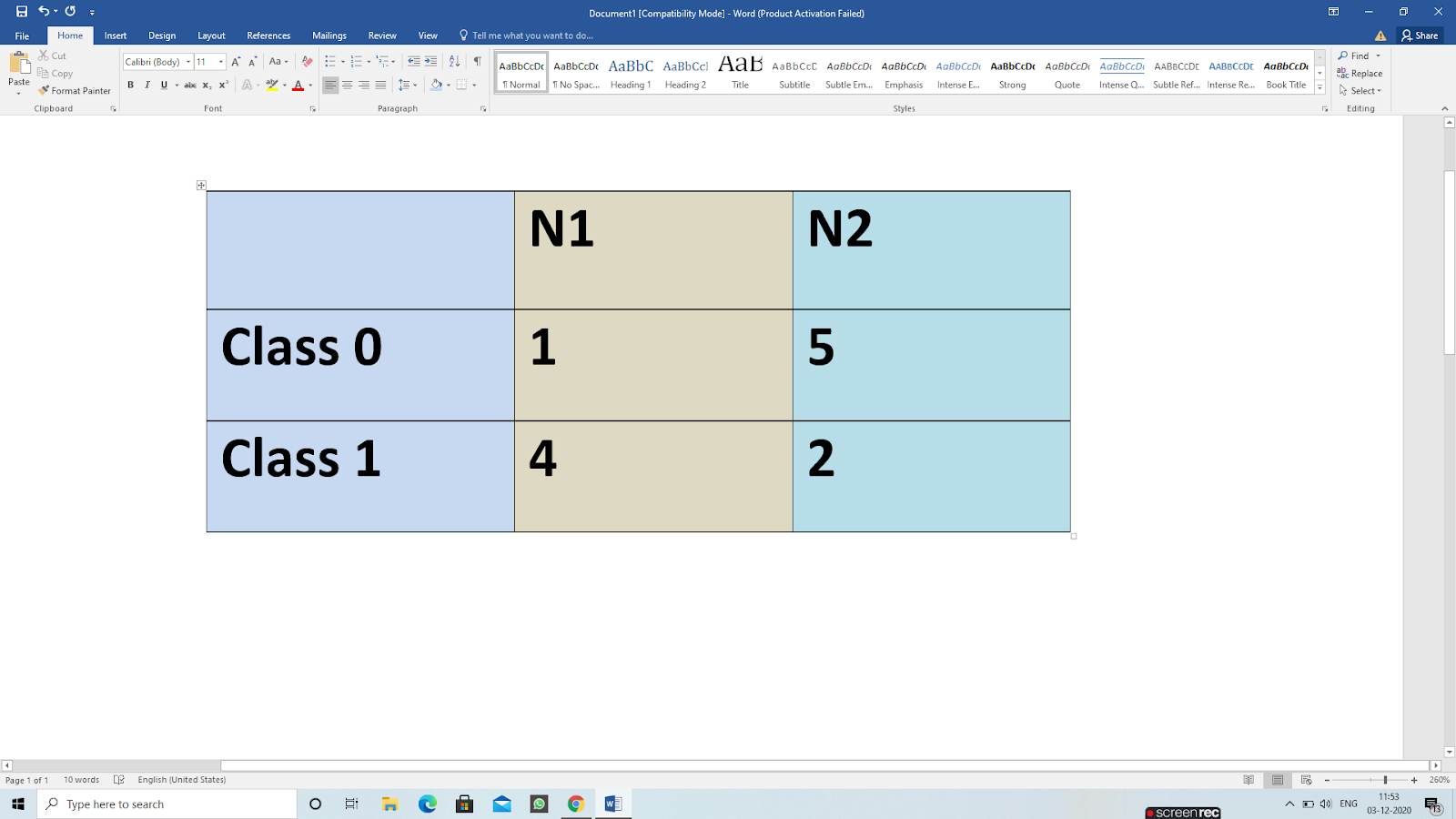
Gini(N1)= 1-[(1/5)2+(4/5)2]
= 1-[(0.2)2+(0.8)2] = 1-[0.04 + 0.64] = 1-0.68 = 0.32
Gini(N2)= 1-[(5/7)2+(427)2] = 1-[(0.2)2+(0.8)2]
= 1-[0.04 + 0.64] = 1-0.6 = 0.32
Gini(children) = (0.32)(5/12)+(0.41)(7/12) = (0.32)(0.416)+(0.41)(0.583) = 0.133+0.239 = 0.372
Conclusion : Classification 2 is our best split by having Gini value 0.372 because which is having the minimum error rate.
Decision Tree Classifier in Scikit-learn:
The Data set I have used to build this classification model is a Movie collection data set.
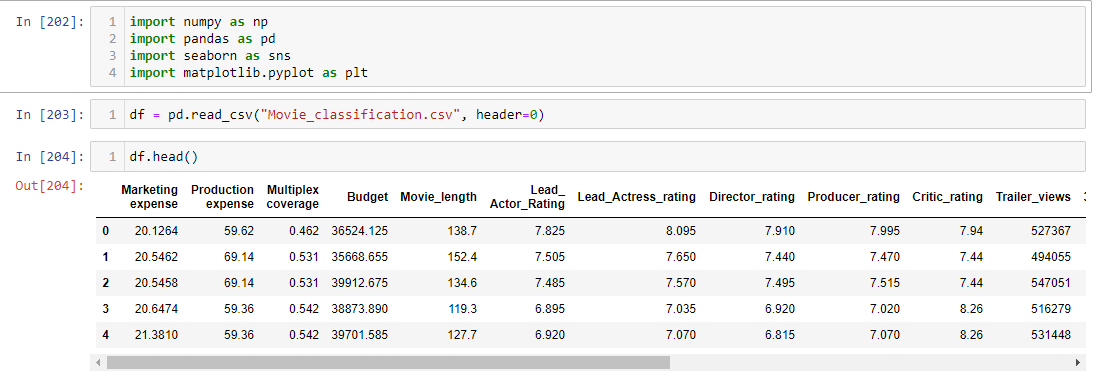
- First Import all the libraries required.
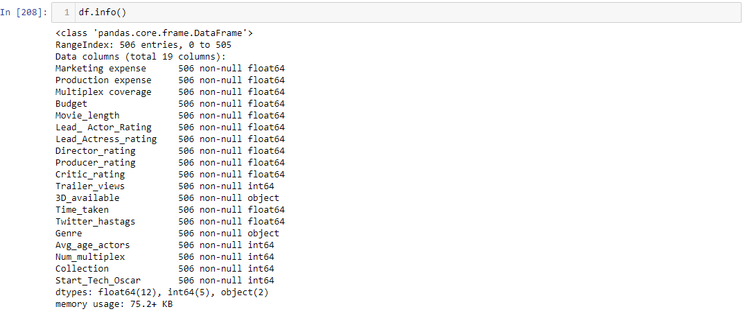
- Import the Movie Classification.csv file and run the data. Load the dataset it consists of 19 columns and 506 rows.
Marketing expense, Production expense, Multiplex coverage, Budget Movie_length, Lead_ Actor_Rating, Lead_Actress_rating, Director_rating Producer_rating, Critic_rating, Trailer_views, 3D_available, Time_taken Twitter_hastags, Genre, Avg_age_actors, Num_multiplex, Collection Start_Tech_Oscar. Our Dependent variable is Collection. We will predict the Collection variable using all the previous data.

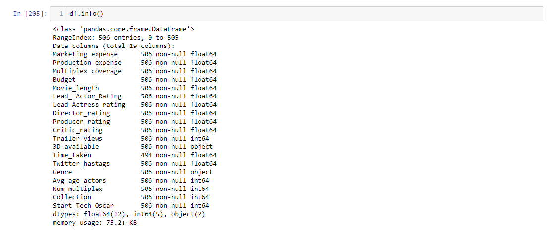
In the below details you can see the count of columns, rows and values present in a single column. In column Time_Taken we can see that there are only 494 values when compared with other columns there are some missing values in that column. I will show you how to treat that missing value further.
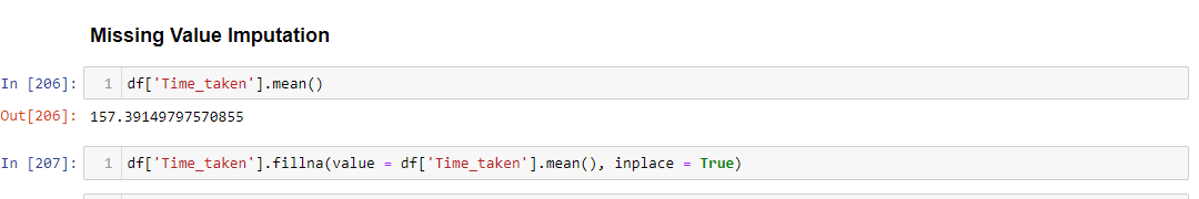
To treat the missing value present in the Time_Taken column we used the mean value of that column to fill the values. So the mean value is 157.39 fill the missing values with the mean value
Now to check whether the missing values are filled or not, use info() function.
.

We have categorical variables in the column “3D_available” and also in “Genre” so we will create a dummy variable on those columns.
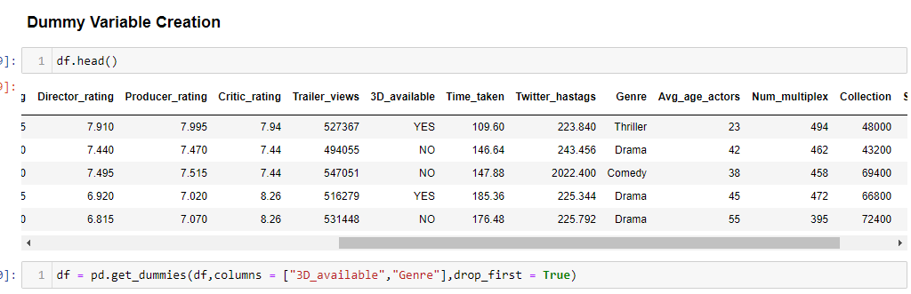
To view whether the values are converted into numerical type use head() Function.
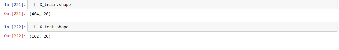

Now we will perform a Test-Train split on the data.


Train the model to perform the Classification Tree.
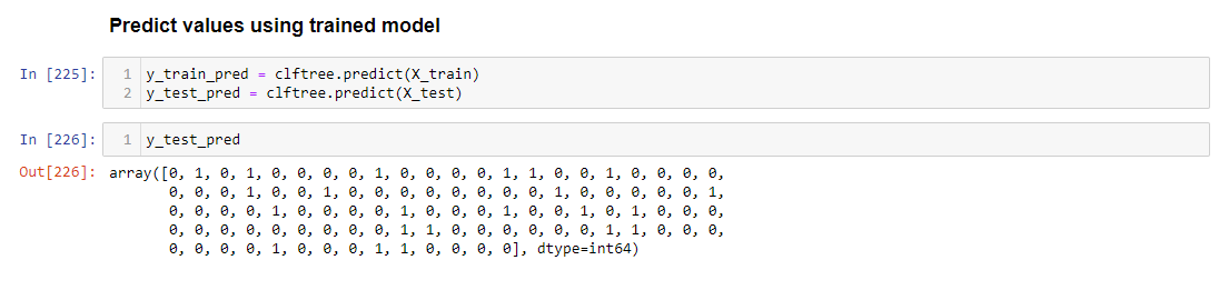
Predicting the values for both Test and Trained Model.
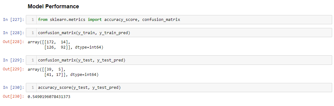
Finding the Model Performance using Accuracy score and Confusion Matrix.

Plotting our Decision Tree Classifier for ”Movie Collection” Data set.

thus, The reason why I only explained Gini and cross entropy is in the above example our Data set classifies the data and creates a decision tree using Gini value.
hence, I hope you understood this blog on Decision trees, Thank you, Happy learning :-).
Written By: Sangamreddy Manasa Valli
Reviewed By: Umamah
If you are Interested In Machine Learning You Can Check Machine Learning Internship Program
Also Check Other Technical And Non Technical Internship Programs