
probability distributions are one of the most important topic for every data scientist. A probability distribution is a function that gives the number of occurrences of the different possible outcomes of the experiment. By observing the probability distribution of samples one can easily recognize the patterns or can make estimations about the population.
There are two types of variables in every dataset:
- Categorical variable
- Numerical variable
Numerical variables are further categorized into two types.
- Discrete random variable: can take only some specific values.
Ex. Die roll, coin toss
- Continuous random variable: can be any real or fractional value in the given range.
Ex. weight, height
Probability Distributions
Probability distribution which has discrete random variables can be describe by probability mass function. however, Probability mass function gives the probability of the occurrence of the variable.
Similarly, probability distribution which has continuous random variables can be describe by probability density function but probability density function does not give the direct probability of the variable. The integration of the probability density function over the range gives the probability of a variable.
There are different types of probability distributions. In this article, we will discuss the 5 most used probability distributions in data science.
1. Normal Distribution:
A normal distribution is one of the most common continuous probability distributions which can thus be find in many real-world phenomena like the height of population, class grade report, etc.
however, A normal distribution is also refer Gaussian distribution. A normal distribution curve is symmetric about the mean. The normal distribution curve shape is the same as that of a bell-shaped curve.
Normal distribution is also represented as N ~ (μ, σ2)
Probability density function for normal distribution is given by

Where μ = mean of the variables
σ2 = variance of the variables
x = random variable


As the standard deviation increases, the normal distribution curve becomes flat with a decrease in density.
Some of the characteristics of a normal distribution are listed below:
- Mode, mean and median values are the same in a normal distribution.
- The integration of the normal distribution curve is equal to 1.
- 68% of the data points lie between the first standard deviation of the mean.
- 95% of the data points lie between the two standard deviation of the mean.
- 99.7% of the data points lie between the three standard deviation of the mean.

Let’s take an example:
suppose your company has 100K employees and you want to order a T-shirt for all employees for a function. however, T-Shirts are available in S, M, L, and XL sizes and Now you want to order a quantity of each size in such a way that most of the employees get the perfect size T-shirt.
Assumption – T-shirt sizes only depend on the height of the employee.
Now obviously you can’t take a measurement of all employees in a short time. So here you can use a distribution for estimating the size of the T-shirt for all employees.
Sampling = here you can take 1000 random employees and measure their height. therefore, get the mean and variance of the employees height and plot the normal distribution curve.
If P(height>=180cm) = 1% then you will have to order a 1000 XL size T-shirt.
If P(160cm>=height<=170cm) = 55% then you will have to order a 55K M size T-shirt.
In this way, you can use a probability distribution of samples to make estimation about the population.
2. Uniform Distribution:
There are two types of uniform distribution.
1. Discrete Uniform Distribution:
When each value of the random variable is equally likely and values are uniformly distributes throughout some interval then that distribution is refer Discrete Uniform Distribution.
so, It is represents as U(a, b), where a is the minimum value and b is the maximum value.
If x is uniformly distribute on the set {a, a+k, a+2k, a+3k up to b}
Then probability of x (P(x)) = k/(b-a+k)
Let’s take an example of a dice throw. Here we have an output set {1, 2, 3, 4, 5, 6} and each outcome has an equal probability of 1/6.

2. Continuous Uniform Distribution:
Continuous uniform distribution thus only takes the a and b value and applies the equal probability density to all values between this range. This forms the shape of a rectangle that’s why this distribution is also refer a rectangular distribution.
The area of the rectangle should be 1.

Let’s suppose the daily sale of the ice cream shop is uniformly distributed with a maximum of 500 and a minimum of 100.
And now you want to find out the probability of sales falling between 200 to 300.
So the probability of a sale falling between 200 and 300 is (300-200)/(500-100) = 1/4.
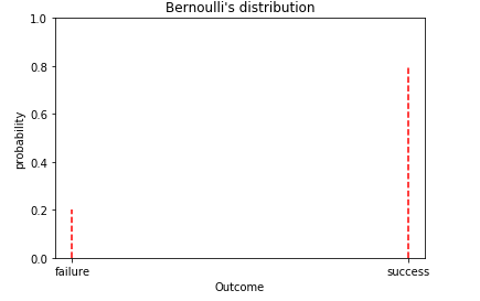
3. Bernoulli’s Distribution:
This is a probability distribution of any single experiment that asks a YES or NO question. Bernoulli’s distribution has only two possible outcomes and that is success and failure or 0 and 1.
The probability of the success or 1 is given by P and the probability of the failure or 0 is given by (1-P).
P(y) = (1- P) for y = 0 or failure
P for y = 1 or success
Let’s take an example,
suppose I am playing a badminton match with Shrikant kidambi. He is a professional player so his chances of winning a match are more than me.
If the winning chances of Shrikant kidambi are 0.8 then the winning chances of me are (1-0.8) = 0.2.
4. Binomial Distribution:
The Binomial distribution can be thought of as the same as that of Bernoulli’s distribution. The only difference is that in Binomial distribution you can consider multiple experiments.
Binomial Distribution is represented as y ~ Bin (n, P)
Where n = number of events
P = probability of success
In Binomial Distribution output of the current experiment does not depend on the previous experiment. The output of each experiment should be either success or failure and the probability of success and failure are the same for all experiments. The Binomial distribution is like a summation of multiple Bernoulli distributions.
Let’s take an example of an unbiased coin toss.
Here the probability of getting head and tail is the same and that is 0.5. Suppose we tossed a coin 10 times then what is the probability of getting a head 5 times out of 10 tosses?
Probability (y=k) = Pk * (1-P)(n-k)
Where n = number of events
P = probability of head outcome = 0.5
y = number of times one got head out of 10
K = 5 and (0<=k<=n)
Probability (y=5) = 0.55 * (1-0.5)(10-5)
Probability (y = 5) = 0.0009765
So the probability of getting 5 heads out of 10 coin tosses is 0.0009765.
5. Pareto Distribution:
Pareto distribution is a skewed distribution with a long tail. It tells that not all the things in the world are evenly distributed. Pareto principle or 80-20 rule states that 80% value can be found at a lower 20% range and the remaining 20% values are distributed over the remaining 80% range.
Example – 80% of the wealth in the world is held by the 20% world population and the remaining 20% wealth is held by 80% of the world population.
Pareto distribution is also represented as Pareto ~ (Xm, α )
The probability density function for Pareto distribution is
P(x) = (ɑ*Xmɑ ) / (X ɑ+1)
Where Xm = location parameter (minimum value of X)
α = slope parameter or pareto index
X = random variable

Pareto distribution is also used in many social, geographical, and real-world phenomena.
Conclusion:
In this article, we have studied the most used probability distributions in data science, their formula, applications with examples, and how we can get insights of the population by observing the distribution of the samples.
written by: Sanket Landge
reviewed by: Rushikesh Lavate
If you are Interested In Machine Learning You Can Check Machine Learning Internship Program
Also Check Other Technical And Non Technical Internship Programs