

What is Machine Learning?
It is a subset of artificial intelligence (AI) that allows the system to automatically learn and improve from experience without being explicitly programmed.
Supervised Learning:
It works as a supervisor or teacher. Basically, In supervised learning, we tend to teach or train the machine with labeled knowledge (that means that knowledge is already labeled with some predefined class). Then we tend to check our model with some unknown new set of knowledge and predict the extent for them.
Learning from the labeled data and applying the knowledge to predict the label of the new data(test data), is known as Supervised Learning.
Types of Supervised Learning:
- Linear Regression.
- Logistic regression.
- Decision Tree.
- Random Forest.
- Naïve Bayes Classifier.
1. Linear Regression:
Regression stands for modeling a target value based on independent variables and Linear Regression is used to find the relationship between a dependent(y) and independent variable(x).
Linear regression is a supervised machine learning algorithm. Always works with continuous value.
Formula: y =mx+c
m=slope of line and c= intercept.
The main target for linear regression to find the best value for X and Y.
Now, let us predict the salary of people based on their experience using a linear regression model or Salary Prediction Model.
Salary Prediction Model
Firstly, import the libraries i.e NumPy and pandas which are used for building the data frames.
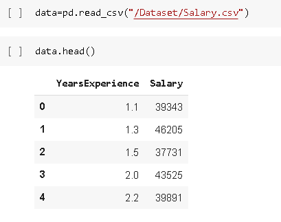
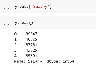
Load the Salary dataset which is in .csv format by using function pd.read_csv and by using .head() we can see the top 5 data of the dataset.
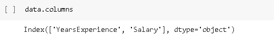
data.columns:
show the name and data type of the columns of the dataset.
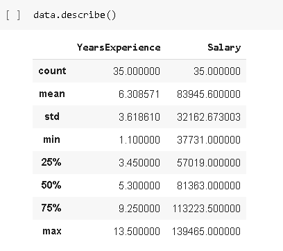
data.describe():
displays the calculated values of gives the total count, mean, standard deviation, minimum, maximum, and also iQR of each column.
If you want to find the null values for each row then by using df.isnull() command it shows the null values of each row from the dataset in boolean form i.e true or false which means the null value is either present or absent in the dataset.

If you want to check the null values for each column then using data.isnull().any() it displays the null values from each column of the dataset in the form of boolean data type i.e true or false.
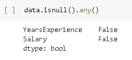
data.isnull.sum():
It is thus a function which will sum the missing values of the columns and displays the result as integer data type i.e 0,1,2,3,…

Now, we are importing the libraries such as matplotlib and seaborn which is use for data visualization which helps to visualize the data from the dataset.
By using the .plot function we can plot the graph using data of two columns from the dataset. For the x-axis, we will take the’ Salary’ column and for the y-axis will consider the column named ‘YearsExperience’.
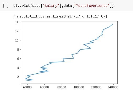
As you can see from the above graph the curve is not smooth i.e there are many variations.
Building the Model:
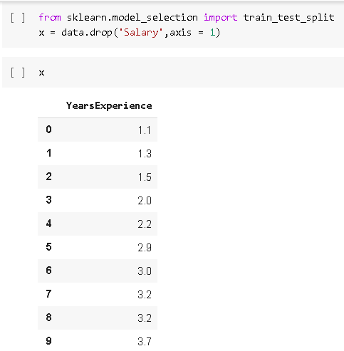
Now, we will import the train_test_split from sklearn which will help us to split our data into training and testing data i.e it will divide the dataset into the training part and testing part because we don’t want to show all the data to our model in the training phase because the model will not able to understand how to react or process the to the new data for predicting the resultant output.
For x we gonna take the independent variable i.e YearsExperience and by using the .drop function we will drop the Salary column from the data frame and then when you print x you will get the data of YearsExperience column only.
For y we are gonna take a dependent variable data which is from the column Salary.
Now, we will split the data as xtrain, xtest, ytrain, ytest and then will consider the x and y values and set the tes_size as 0.2 which means we will consider only using 20 % of data for the testing phase and the rest 80 % data for training the model. By setting the random_state as 42 it will take any data for training and testing from the dataset.

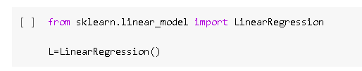
Import LinearRegression from sklearn and then will call our linear regression function.
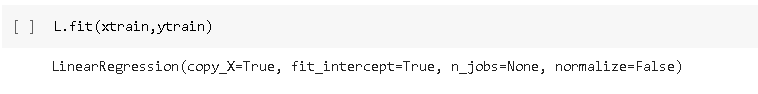
Then we will fit the model using the .fit function and will provide xtrain and ytrain. After that, as you see in the output our model gets trained.
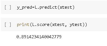
Now, if we want to do the prediction then we will take xtest data along with the .predict function and then print the y_pred to get the prediction data. And for the accuracy score, we will use the .score function and consider the data of xtest and test. As you can see our linear regression model accuracy is 0.8914 i.e 84 %.
CONCLUSION:
Simple linear regression helps us to predict a dependent variable from an independent one, on continuous data of the data frame. The regression line is vital because it makes the estimation of a variable a lot correct for Salary Prediction Model. it permits the estimation of a response variable for people with values of the carrier variable not enclosed within the knowledge.
written by: Kanchan Yadav
reviewed by: Rushikesh Lavate
If you are Interested In Machine Learning You Can Check Machine Learning Internship Program
Also Check Other Technical And Non Technical Internship Programs