
In Supervised Machine Learning, there are two types of problems. One is Classification and the other one is Regression. The data scientists train algorithms with the training dataset to build different models and select the best model based on performance. There are certain evaluation matrix in Classification and regression based on which the best model is selected.
In regression, the target variable is continuous and in classification, the target variable is discrete or categorical. Therefore, there are different evaluation criteria based on which the best model is selected in these two types of supervised machine learning.
Today I will be discussing the various evaluation matrices used in classification and regression.
Evaluation Matrix in Classification
The following are the evaluation matrices when the output variable is categorical or discrete.
1. Confusion Matrix:
It is a 2*2 matrix that shows four different combinations of actual value and predicted outcome. This is used for binary classification problems.

The above fig is a representation of a confusion matrix. It has four elements which are as follows:
- True-positive (TP): The predicted outcome is positive when actually it is positive.
- False-negative (FN): The predicted outcome is negative when it is actually positive.
- True-negative (TN): The predicted outcome is negative when actually it is negative.
- False-positive (FP): The predicted outcome is positive when actually it is negative.
Based on the above elements’ different evaluation terms like accuracy, Recall, precision, specificity, F1-Score are calculated and used for selecting models depending on the business scenario.
2. Accuracy:
It is defined as the ratio of correct predicted values to the total number of predicted values. Corrected Predicted values include both positive and negative values which are predicted correctly.
Accuracy= Corrected Predicted values/ Total Predicted values
From the above confusion matrix,
Accuracy = (TP+TN)/(TP+TN+FP+FN)
The value of accuracy ranges from 0 to1. A value closer to 1 indicates a better model.
Or Error = 1- Accuracy
In reality, for unbalanced data, measuring model performance on accuracy is not a great idea. For this reason, other measures are available which we will discuss next.
We will first have a glance at the following terms.
True Positive Rate or TPR: The ratio of actual positive predicted values to the total actual positive values. The range varies from 0 to 1. The higher the value the better is the model. This is also called Sensitivity.
TPR = TP/(TP+FN)
False Negative rate or FNR: The ratio of actual positive, predicted as negative to total actual positive values. Lower the FNR better is the model. This is also called 1- Sensitivity
FNR = FN/(TP+FN)
True Negative Rate or TNR: The ratio of predicted negative values that are actually negative to the total actual negative values.
TNR= TN/ TN+FP
It is also refer specificity. The higher the value the better is the model.
False Positive Rate or FPR: The ratio of actual negative, predicted as positive to the total actual negative values.
FPR =FP/ TN+FP
It is known as 1- Specificity. Lower the value of FTR better is the model.
3. Recall:
Out of all actual positive values, how many are actually predicted positive.
Recall =Predictions positive/Total Actual Positive
Recall = TP/TP+FN
4. Precision:
Out of total positive predicted values how many are actually positive
Precision= Predictions Actually Positive/ Total Predicted Positive
Precision= TP/(TP+FP)
Precision and Recall are select as evaluation matrix depending on business scenario
5. F1-Score:
This is a combination of precision and recall. It can be define as the harmonic mean of precision and recall.
The Formula for F1-score is
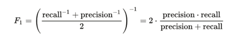
The value ranges from 0 to 1. F1-score is maximum when Precision = Recall
6. AUC-ROC Curve
This a graph between True Positive rate and False Positive Rate.
AUC stands for Area Under the Curve
ROC stands for Receiver Operating Characteristics. It’s an evaluation matrix for binary classification. It gives a tradeoff between True Positives and False Positives.

In the above curve, the shaded region is the Area Under Curve. The greater the area the better is the model. The dashed line covering 50% of the area. For any good model, the score should always be above the dashed line. You will be clearer from the following figure.

Evaluation Matrices in Regression
The following are the matrices used when the target variable is continuous.
1. Mean Absolute Error
Error is defined as how far the predicted values from the actual observe values. The lesser the error better is the model which means predicted values are closer to the actual values
Error = Actual values – Predicted values
Consider the following table. It is showing the actual values, the predicted values, and the error is thus calculate for each instance based on the above formula
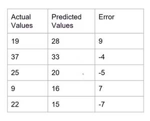
Total Average error is calculate by adding all the errors and then dividing the value by the number of instances.
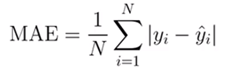
But we can see that there are negative errors along with positive errors. So, the negative errors and positive errors cancel each other and give a final value that is very less. So, it will be very difficult to determine the actual error. For this reason, the absolute difference of error is consider, and the Mean Absolute Error is calculate.
The Mean Absolute error formula is consider below.
2. Mean Square Error
The other way of getting rid of the above problem is squaring the error and then taking the average which is named as Mean square error.
The mathematical expression for Mean Square Error is mention below.

3. Root Mean Square Error (RMSE)
The problem with mean square error is that, since the error value is squaring, so units are also getting square. It is not precisely representing the errors. Therefore, the root of the MSE is consider so that unit turns into normal form.
Mathematically it can be represent as,

4. R-Squared and Adjusted R-Square
In the linear regression model, R-Square is define as the measure of the proportion of variation of the independent variable explained by the dependent variables. It refer as the coefficient of determination.
Mathematically R-square can be display as

where, SSRes = Residual Sum of squared error. And SSTOT = Total Sum of Squared error
The value ranges from 0 to 1. The higher the model the better is the model.
Generally, the model having R2 > 0.8 can be consider as a good model.
Adjusted R-Square is the same as R-Square used in the case of Multi Linear Regression.
It is the measure of the proportion of variation of the independent variable explain by the dependent variables which are significant.
The adjusted R-Square value can be lesser than or equal to the R-Square value. If more variables are add up, then the R2 value will increase but the adjusted R2 value will only increase if the variables are significant.
Conclusion
In this article, I have discussed different evaluation matrices for classification and regression models in brief. Hope it is clear.
Thank you for reading the article. Hope to receive your comments and suggestions.
Written By: Nabanita Paul
Reviewed By: Krishna Heroor
If you are Interested In Machine Learning You Can Check Machine Learning Internship Program
Also Check Other Technical And Non Technical Internship Programs