
Neural networks is the most active field of research in Machine learning these days simply because of the ability of the neural networks to learn highly complex and nonlinear functions. Neural networks also play a critical role in Deep learning. How so? That is for sure a deep question (pardon the pun). Neural networks are the units that do all the “hard work”. While they may seem like a box, deep down (sorry once again), they are making predictions like any other model in Machine learning. Let’s see in a bit detail
Why Neural Networks?
The term Neural network was coined from the human brain. The human brain is a powerhouse of energy and is able to do a lot of tasks with great intricacy and accuracy. This inspired a lot of people to figure out how the human brain exactly works.
The human brain contains billions of neurons which are intricately interconnected. These different neurons are simple computing units, but together, they have the ability to perform extremely complex tasks.
Certain features of neurons have been included during the process of formation of the neural networks. They are
- Massive parallelism: There consists of many units which are simple individually but they work hand in hand to achieve complex tasks.
- Connectionism: They are interconnected very minutely with each other, and thus a task can be solved together.
- Model distributed Associative Memory: This modelling can be achieved with the help of weights in the synaptic connections.
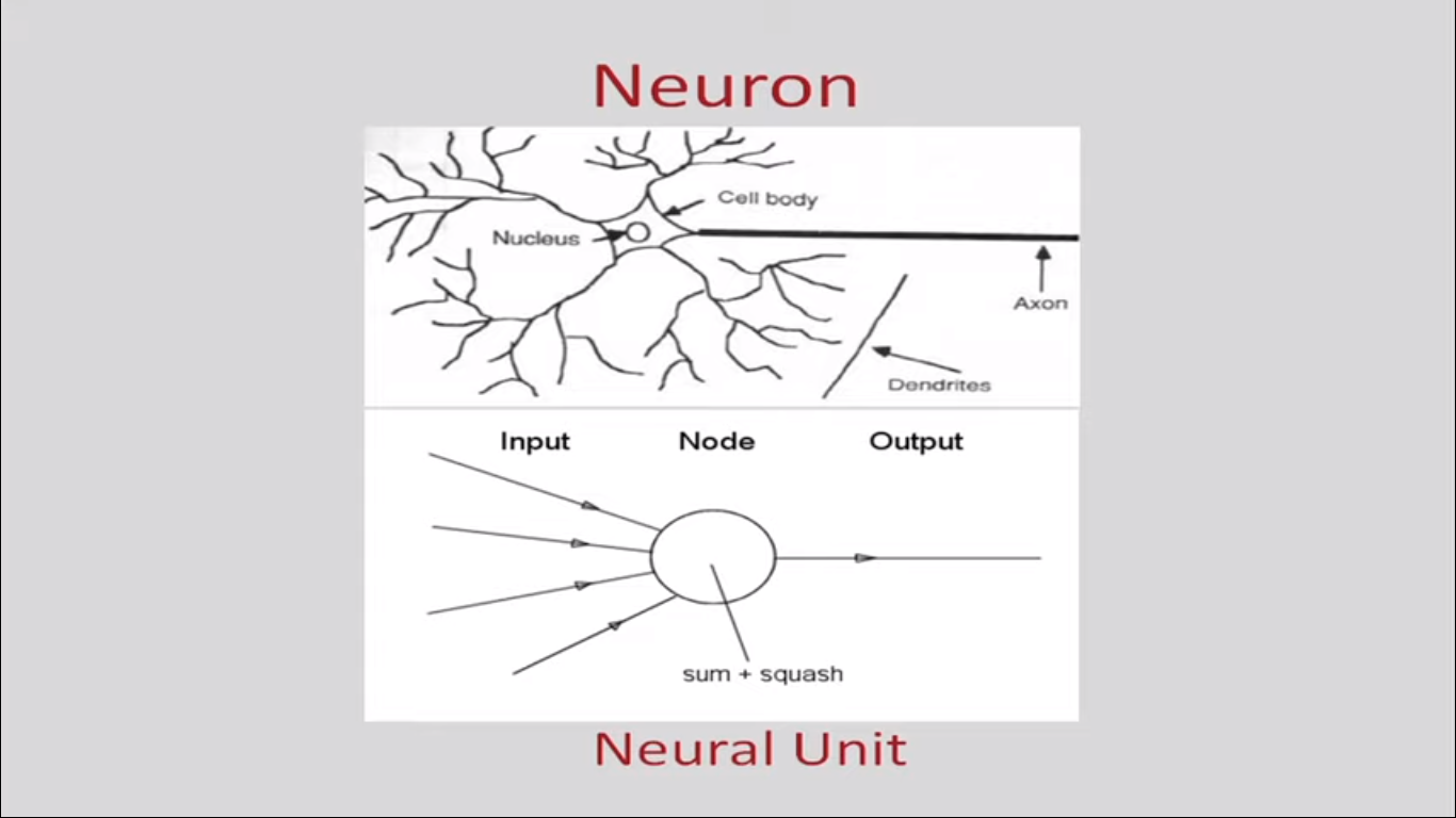
FIG 1: ACTUAL NEURON AND NEURAL UNIT
As it can be seen the cell body consists of nucleus and the tentacles type objects are dendrites through which input is accepted and from axon the output is given. This can be replicated as a neural unit in Machine learning, comprising of inputs, followed by computation at the node and hence the output. The weighted some of the inputs is found out and applies a function like the sigmoid function etc.

In the figure it can be seen that the output from the axon of Neuron A feeds into the input of Neuron B with the help of synaptic connections through dendrites. This inspired the neural network architecture.
Single Layer Neural Network
The primitive unit in a neural network is perceptron. It consists of N inputs.
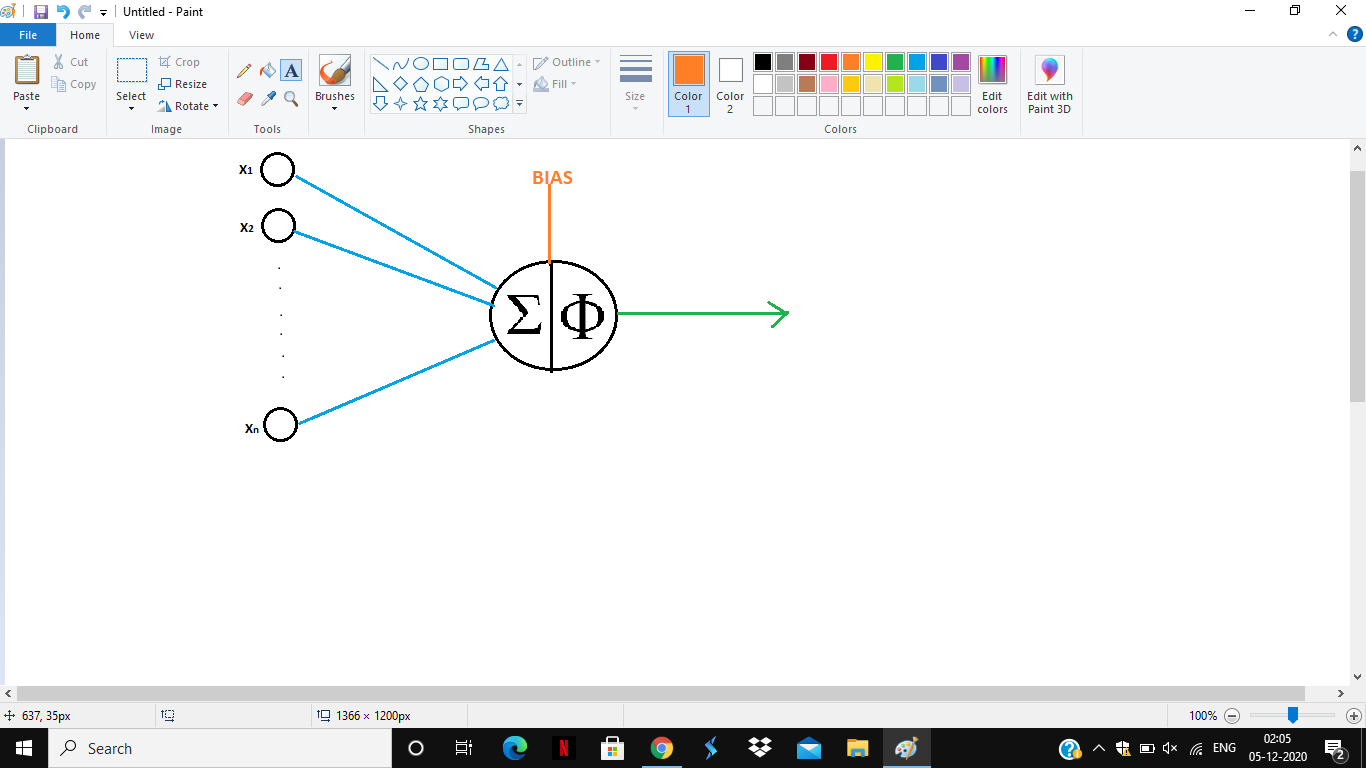
There are 2 parts, first a weighted summation of input is calculated. There is another input termed as bias. The combined input is passed through another transfer function denoted by Φ. For a linear unit Φ(z)=z. In other words, just the summation is passed and this is known as the linear transfer. For a linear transfer at the summation region,
y=i=1mwixi+B
Where B is the value of the fixed bias and wi refers to the respective weights of xi. If B=W0X0 such that X0 is 1 then the summation can be rewritten as
y=i=0mwixi
Using supervised learning, the single layer neural network can be trained. Here training refers to learning the values of weights that is, w0,w1,w2,…wN so that the network has a good fit for the training examples.
Perceptron Training Rule
In this type of training rule, when this network is setted up, there are some initial values of the weights, and after each iteration, the weight is updated. In the simplest training rule, each example is fed one at a time to this network. Based on how the network performs, the weight is updated. The updation of weight is given as
wi=wi+wi
wi= (y-y)xi
Here y is the target output (what we want), and yis what is obtained output (what we get) from the network. A particular example is fed, which consists of different components (x1,x2…xn) corresponding to the different features. If the target output equals obtained output then wi=0 and in this case no change in weight is required. But if the value of (y-y) are different, then the weight needs to be updated.is known as the learning weight.
If a number of examples are taken and are fed one by one, it can be observed that the perceptron based learning converges to a model being consistent provided D (the training example) is linearly separable. If such a linear separation surface exists, by applying this perceptron training rule, the learning algorithm will converge to a hypothesis which will classify the training data set.
But if the training example is not linearly separable , then this algorithm will not converge. In those cases the gradient descent algorithm is used and is applied for more general cases. If in a scenario, with respect to a particular value of the parameters, the errors can be defined, then gradient descent can be performed on this error function, to obtain that value of the parameters for which this error function is minimised.
Limitations of Perceptron
- Perceptrons have the property of monotonicity which is a big problem in perceptrons. If for example, the link consists of a positive weight, activation could only increase as the value of the input increases (irrespective of other input values). Thus those functions in which input interactions cancel each other cannot be represented by the perceptron. This means it is unable to handle the interactions between the network.
- It is also unable to represent those functions where interactions of the input cancel one another’s effect (for eg XOR).
The solution to this is the multi-layer neural network.
Multi-Layer Neural Network
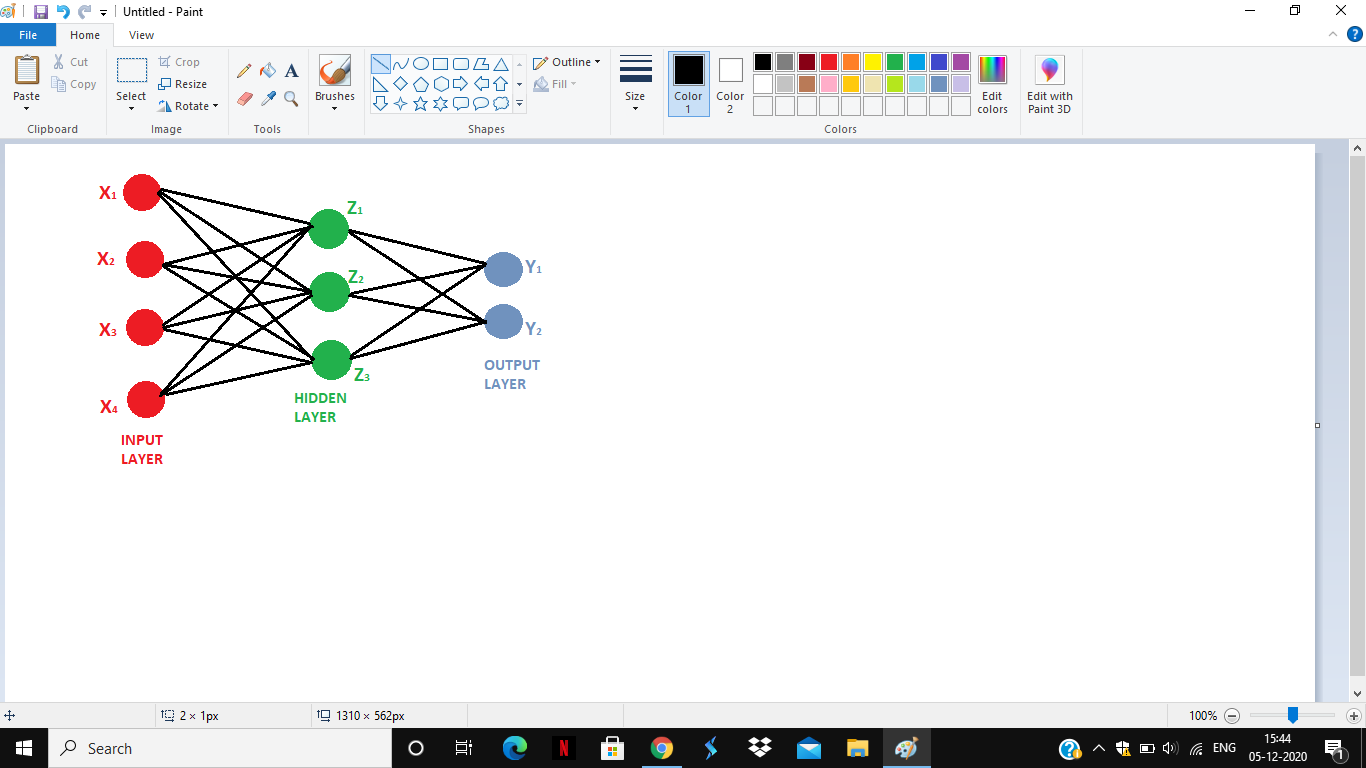
The units in the MLN network are stacked on each other. In this there is one input layer (X layer) and one output layer(Y layer) ,and between the input and the output layer, there are hidden units(Z layer). The reason for calling them hidden is because in the training examples they are not observed.
With the help of hidden units, many nonlinear functions can be represented.
General Structure of Multilayer Network
The figure above shows the general structure of the Multilayer Network. The components of any layer can be of any number. If the connections (the black lines) are unidirectional then the MLN is known as Feed Forward Neural Network. That is there cannot be any arrow which points from the hidden layer to the Input layer. This structure is called a layer structure.
Like in the perceptron based training, depending upon the error in the output, the weights were modified so that error was reduced. However there is one issue here. At the output layer, the value of the weights were known as so the output layer can be modified. But at the hidden layers, the ideal output is not available or given to us. So on what basis, the weights of the hidden layer be computed?
to avert this problem, the error observed at the output layer is propagated or directed backwards. Thus MLN works on the assumption that error at the output layer is due to the result at the hidden layer. If there were more hidden layers, then these errors would be further back propagated. Therefore the computation in the MLN is forward while the error signals flow backwards. This algorithm for updating weights using error signals is known as Back Propagation Training Algorithm.
Back Propagation Training Algorithm
The algorithm involves the following steps
STEP 1: Initialisation
The weights and the levels of threshold of the networks are setted to random numbers which are uniformly distributed within a small range
STEP 2: Forward Computing
An input vector X is applied to the input units and the activation/output vector Z on the hidden layer is computed. This is given as
zj=(ivi j xi)
The output vector Y on the output layer is computed
yk=(iwjk zj)
Y is the result of computation. Here v is the weights of the hidden layer and w is the weights of the output layer.
STEP 3: Update the weights
This step includes updation of weights in W with the help of gradient descent. This is not applicable to updating v (between input and the hidden) as one does not know the target values of hidden layer units. The solution is backpropagation. This error can be computed as explained below.
- For a single output neuron, the error function is given as
E=12(y-y)2
For each unit j, the output oj is defined as
oj=(netj)=(k=1nwjk ok)
The netj input to the neuron is the weighted sum of outputs ok of previous n neurons. The derivative of the error is
Ewi j=Eo jojnet jnetjwi j
l(Eo jojnet zl wj zl)(netj) (1-(netj)) oi
Ewi j=j oi
j=Eo jojnet j={(z zl) oj (1- oj) …(2)(oj – yi)oj(1 – oj) …(1)
Equation 1 is used if j is the output neuron.
Equation 2 is used if j is the inner neuron.
If the weight wi,j needs to be updated using the gradient descent, a learning rate must be chosen.
This brings us finally to
wi=Ewi j
This can be propagated further if there are more hidden layers.
Expressiveness of Multilayer Network
The multilayer network is able to represent the interactions among the inputs unlike the single layer Network. Also, Two layer Networks is able to represent any Boolean function and for that matter any continuous functions (within a tolerance limit) if the number of hidden units are sufficient and suitable activation functions are used. However, the next question that comes is whether the function is learnable or not?
however, There is the existence of a learning algorithm but the guarantees are weaker than the perceptron based learning algorithms. Like in perceptron if it was stated boldly as if a function exists then the given procedure will converge. However for MLN, such bold statements cannot be made, but research is being done extensively in this field.
written by: Aryaman Dubey
Reviewed By: Krishna Heroor
If you are Interested In Machine Learning You Can Check Machine Learning Internship Program
Also Check Other Technical And Non Technical Internship Programs