
A Brief Introduction to RNNs
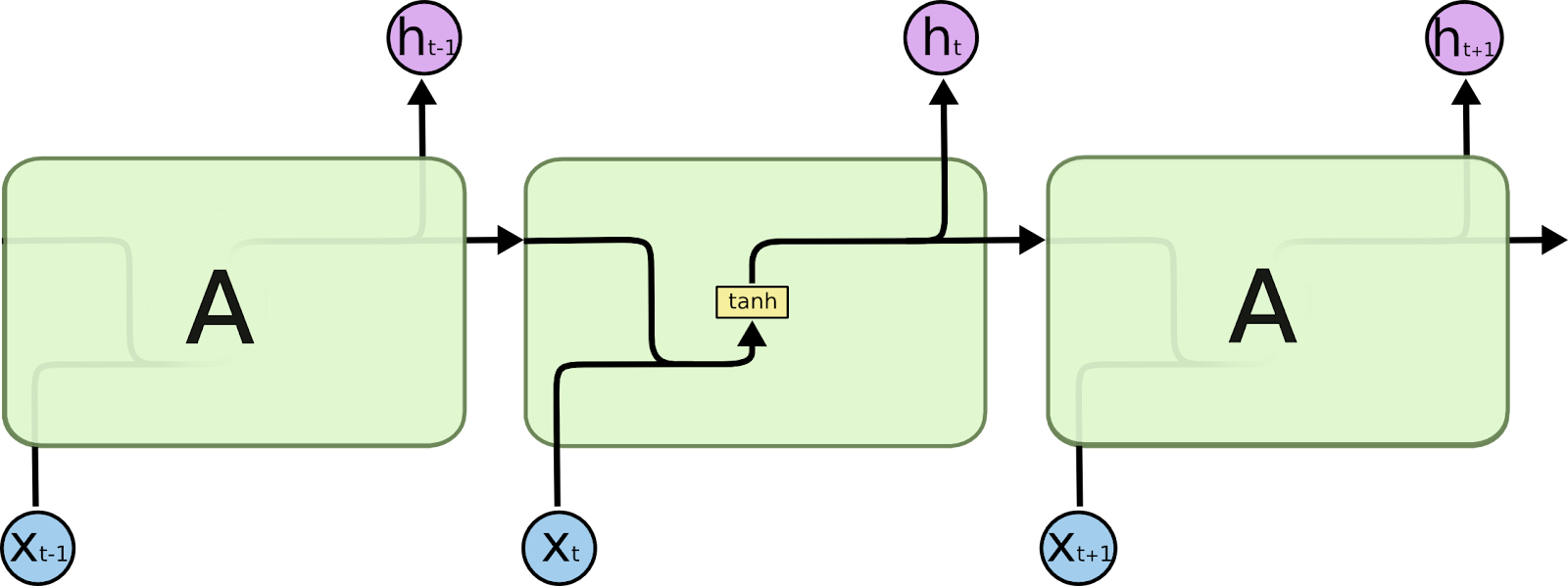
Image courtesy: Understanding LSTM Networks from colah’s blog
Before we can understand what LSTMs are, We need to have an idea about RNNs, which is a basic building block for LSTMs. RNNs(Recurrent Neural Networks) is a type of NNs which are capable of working on data that has a lot of input features. You might be thinking what’s the problem with conventional DNNs. When the input layer is very large(let it be 108 units).
even if the first hidden layer has 100 units, the parameters that need to be learned are very high(that is 1010). This can take a long time leaving the network inefficient. An example of such a situation is NLP(Natural Language Processing), where the dictionary to be learned may vary from thousands to millions of words. On the other hand, RNNs have a different architecture where each layer has units equal to the features(words in a dictionary) and then each element of the sequence is fed to each hidden layer. These layers have ‘tanh’ activations. Each
hidden layer receives the activation of its previous layer and uses both activations from the previous layer and input to predict. This creates a network in which every layer has information about its previous layers and can hence recognize sequences. Although the previous layers do not have information about future layers, this can be solved using a BRNN(Bi-directional Recurrent Neural Network).
What are LSTM Networks?
LSTM abbreviated as Long Short Term Memory is an architecture type of RNN(Recurrent Neural Networks). The hidden layers of LSTM networks are similar to that of RNNs but they have some key differences.
Image courtesy: Understanding LSTM Networks from colah’s blog
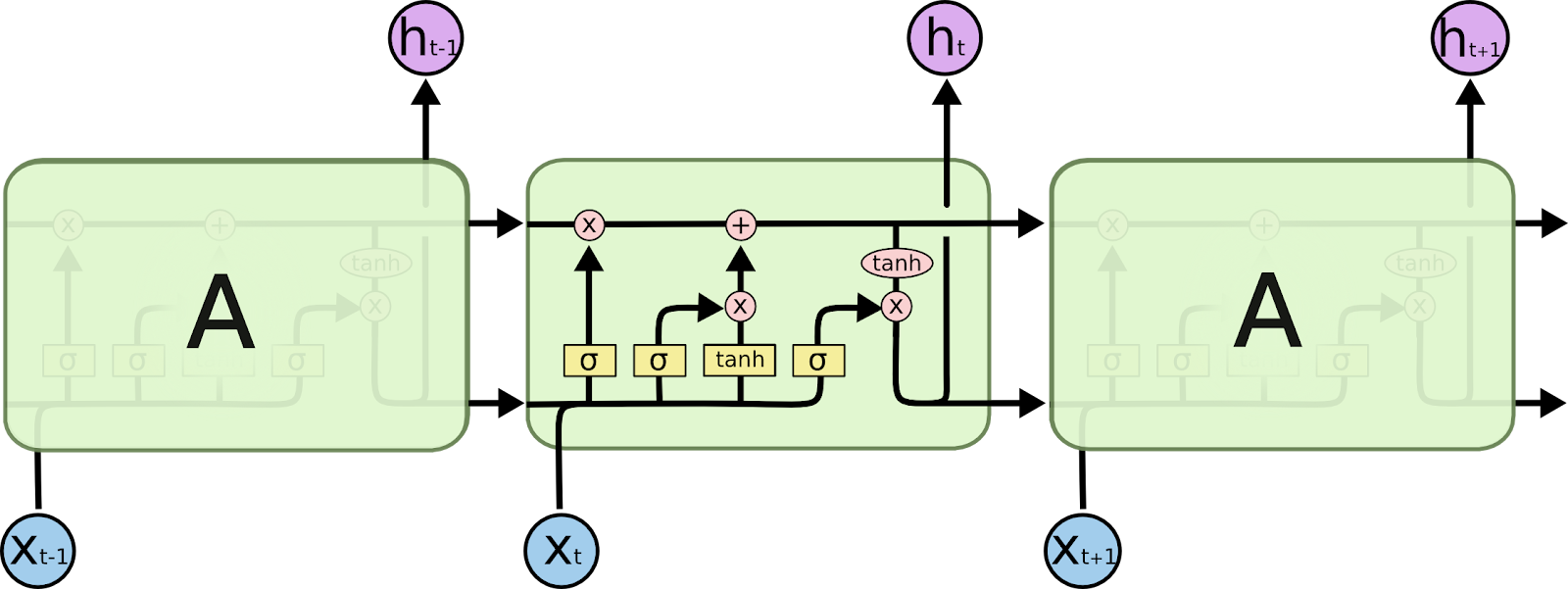
- Instead of having just the activations for the next and output layer, they also have certain cells, which are used to store certain information about inputs.
- Apart from this, there are three gates, which determines if the information is to be stored or not.
Why LSTMs, not RNNs?
Although RNNs are quite good at a lot of applications, the information throughout the network gets lost, if the network is very deep. This is caused because of something called Vanishing Gradient. Vanishing Gradient occurs when the value of the Gradient becomes approximately zero through backpropagation.
an important step in optimizing Neural Networks. When the network is very deep, for RNNs, the information gets lost soon after a few hidden layers. This makes them inappropriate for applications such as Text Prediction and Time Series Forecasting. Thus we need networks where each hidden layer stores its values for future use, achieved by LSTMs.
How do they work?
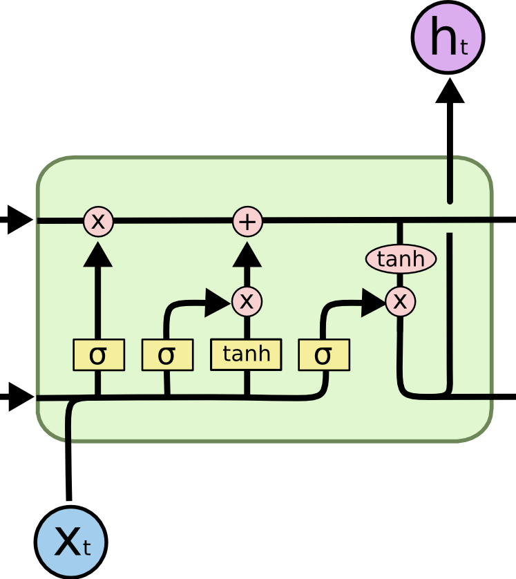
As mentioned earlier, each hidden layer is introduced with a new variable called cell denoted by ‘c’ which will store some information about the inputs. The cell has ‘tanh’ activation, and its weights and bias(denoted by Wc and bc). There are two gates called update gate and forget gate(denoted by greek alphabet gamma). There is one final gate called the output gate. These gates have ‘sigmoid’ activations and hence they determine whether the information should be stored or not.
The LSTM works on a set of equations that defines its structure.
c<t>= tanh (Wc[a<t-1>, x<t>] + bc)
u= (Wu[a<t-1>, x<t>] + bu)
f= (Wu[a<t-1>, x<t>] + bf)
o= (Wo[a<t-1>, x<t>] + bo)
c<t>=u*c<t>+f*c<t-1>
a<t>=o*tanh (c<t>)
Activation of the update gate will allow the cell to store and similarly, activation of the forget gate allows it to retain the old value (Note that the gates can have values (0,1) as they have sigmoid activations). Unlike GRUs(Gated Recurrent Units),
they have separate gates for both previous and current value hence both values can be retained. Activation to the next layer depends on the output gate which can be set as well. This creates a flexible network with high controllability.
Implementation with Python(Keras)
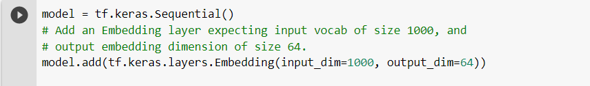
We can start by importing the Deep-Learning Keras Library.
LSTM constructor is stored under ‘tensorflow.keras.layers’. Given below all the instantiating parameters that can be initialized during the creation of an LSTM layer. Although a few of them are used generally.

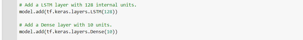
We will start making a simple LSTM network by initializing the model. Then, we are going to make an embedded layer that will act as the dictionary from which the network will learn.
Then we will add the required number of hidden LSTM layers, followed by a dense network that will serve as the output layer.
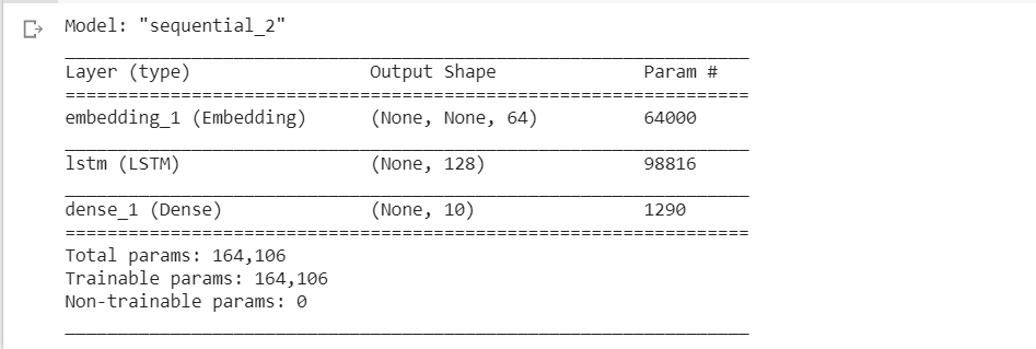
Finally, we will call the model.summary() to show all the layers together and cross verify the structure.
This shows the Layer type, Output shapes, and Parameters of each hidden layer in this LSTM network.
Conclusion on LSTM:
We have seen what RNNs are, why they are important, and what are their drawbacks. Then we saw LSTM layer architecture that replaced the conventional RNNs layers and solved its drawbacks. Practically we use BRNNs with LSTM/GRU hidden layers.
These networks learn to solve a lot of real-world problems such as Speech Recognition, Machine Translation, Time-Series Forecasting, etc. Considering the importance of AI in this decade, we need to educate ourselves more about the role of AI in our lives. Their applications are infinite and can be used in almost every field, where problems exist
Acknowledgment
I have learned whatever I know about LSTM networks from the course Sequence Models from deeplearning.ai. The blog Understanding LSTM Networks has also helped me a lot to write this blog as it is very informative about its working. Besides this, you can also refer to the paper Long Short-Term Memory by Sepp Hochreiter and Jürgen Schmidhuber for more detailed information about these networks.
written by: Soumya Ranjan Acharya
reviewed by: Rushikesh Lavate
If you are Interested In Machine Learning You Can Check Machine Learning Internship Program
Also Check Other Technical And Non Technical Internship Programs