
This article aims to design a simple one hidden layer Linear RNN from scratch to count the number of ones in a binary sequence ( e.g., number of ones in [ 1, 1, 1, 0, 0, 1, 0, 0, 1, 1] is 6)
The structure of Linear RNN and corresponding equations are given as follows:
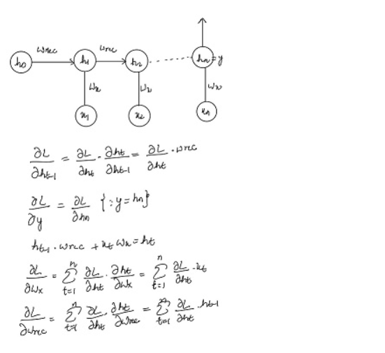
Note 1: There are no non-linear activation functions in this architecture to make backpropagation of gradients simple.
Note 2: The last timestamp’s hidden state is the output of the network.
To do | Linear RNN From Scratch
- Perform forward and backward pass. so, You cannot use gradient tape in TensorFlow (or equivalent in PyTorch). (4+6 = 10 points)
- so, Use mean square error for computing loss and plot the mesh-grid of the loss surface (w_x vs. w_rec). (3 points)
- thus, On this loss surface, mark points (w_x, w_rec) that show exploding and vanishing gradients property. (2 points)
- Give an insight into the instability of gradients during backward propagation on a graph. then, Plot a graph between gradients of loss w.r.t hidden state at time t (Y-axis) and timestamps t (X-axis). Note that you have to plot for various (w_x, w_rec) showing peculiar properties from the previous question. Mark your observations. (5 + 3 = 8 points)
- so, Use Rprop (Resilient Propagation) as an optimization algorithm; you can also use the library (if any) for this part. (3 points)
- thus, Plot the optimization trajectory on the loss surface. (2 points)
- Is your Linear RNN well trained? Does it count the number of ones in the binary list well? thus, How significant a change is observed in model training by introduction of Resilient Propagation? (2 points)
Now we will follow the following steps:
Step 1: Import relevant library
| # Importsimport numpy as np import matplotlibimport matplotlib.pyplot as plt from matplotlib import cmfrom matplotlib.colors import LogNormimport seaborn as snssns.set_style(‘darkgrid’)np.random.seed(seed=1) #So than random number once assigned don’t change |
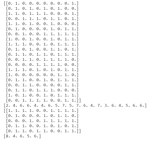
Step 2: Generate synthetic dataset
| # Following code snippet generates a binary sequence. samples = 20sequence_len = 10#Train Sequencestrain_X = np.zeros((samples, sequence_len))for row_idx in range(samples): train_X[row_idx,:] = np.around(np.random.rand(sequence_len)).astype(int)print(train_X) train_Y = np.sum(train_X, axis=1)print(train_Y) #Test SequencestestX = np.zeros((5, sequence_len))for row_idx in range(5): testX[row_idx,:] = np.around(np.random.rand(sequence_len)).astype(int)print(testX) testY = np.sum(testX, axis=1)print(testY) |
Step 3: Perform forward and backward pass | Linear RNN From Scratch
| # Compute State k which is equal to current state(xk) and previous state(yk) by multiply recursive weights (wRec) and input weight(wx) def update_state(xk, yk, wx, wRec): return xk * wx + yk * wRec # Performs the forward passdef forward_states(X, wx, wRec): # S matrix will holds all states for all input sequences S = np.zeros((X.shape[0], X.shape[1]+1)) for k in range(0, X.shape[1]): S[:,k+1] = update_state(X[:,k], S[:,k], wx, wRec) return S # Performs the backward passdef backward_pass(X, S, grad_out, wRec): gradient_over_time = np.zeros((X.shape[0], X.shape[1]+1)) gradient_over_time[:,-1] = grad_out wx_grad = 0 wRec_grad = 0 for k in range(X.shape[1], 0, -1): wx_grad += np.sum( np.mean(gradient_over_time[:,k] * X[:,k-1], axis=0)) wRec_grad += np.sum( np.mean(gradient_over_time[:,k] * S[:,k-1]), axis=0) gradient_over_time[:,k-1] = gradient_over_time[:,k] * wRec return (wx_grad, wRec_grad), gradient_over_time # Output gradientdef output_gradient(y, t): return 2. * (y – t) |
Step 4: Use mean square error for computing loss
| # mean square errordef loss(y, t): return np.mean((t – y)**2) |
Step 5: Plot the mesh-grid of the loss surface (w_x vs. w_rec).
On this loss surface, mark points (w_x, w_rec) that thus show exploding and vanishing gradients property.
| # Plotting functions # Points to annotate (wx, wRec, color)points = [(2,2,’k’),(2,1,’r’), (1,2,’w’), (1,1,’m’), (1,0,’c’), (1,0.5,’g’), (1,-0.5,’b’),(-2,-2,’y’)] def loss_surface(wt1_low, wt1_high, wt2_low, wt2_high, nb_of_ws, loss_function): wt1 = np.linspace(wt1_low, wt1_high, num=nb_of_ws) # Weight 1 wt2 = np.linspace(wt2_low, wt2_high, num=nb_of_ws) # Weight 2 ws_1, ws_2 = np.meshgrid(wt1, wt2) # Generate grid loss_ws = np.zeros((nb_of_ws, nb_of_ws)) # Initialize loss matrix # Assign loss matrix with appropriate weights for i in range(nb_of_ws): for j in range(nb_of_ws): loss_ws[i,j] = loss_function(ws_1[i,j], ws_2[i,j]) return ws_1, ws_2, loss_ws def plot_surface(ax, ws_1, ws_2, loss_ws): surf = ax.contourf( ws_1, ws_2, loss_ws, levels=np.logspace(-0.2, 8, 30), cmap=cm.viridis, norm=LogNorm()) ax.set_xlabel(‘$w_{x}$’, fontsize=12) ax.set_ylabel(‘$w_{rec}$’, fontsize=12) return surf #plot the given points.def plot_points(ax, points): for wx, wRec, c in points: ax.plot(wx, wRec, c+’o’, linewidth=2) #For given points plot the loss surfaces togetherdef loss_surface_figure(loss_function, points): fig = plt.figure(figsize=(10, 4)) # Plot figures axis_1 = fig.add_subplot(1,2,1) # Plot overview for loss function ws_1_1, ws_2_1, loss_ws_1 = loss_surface( -3, 3, -3, 3, 100, loss_function) surface_1 = plot_surface(axis_1, ws_1_1, ws_2_1, loss_ws_1 + 1) plot_points(axis_1, points) axis_1.set_xlim(-3, 3) axis_1.set_ylim(-3, 3) axis_2 = fig.add_subplot(1,2,2) # Plot zoom of loss function ws_1_2, ws_2_2, loss_ws_2 = loss_surface( -0.1, 2.1, -0.1, 2.1, 100, loss_function) surface_2 = plot_surface(axis_2, ws_1_2, ws_2_2, loss_ws_2 + 1) plot_points(axis_2, points) axis_2.set_xlim(-0.1, 2.1) axis_2.set_ylim(-0.1, 2.1) fig.subplots_adjust(right=0.8) # Show the colorbar c_ax = fig.add_axes([0.85, 0.12, 0.03, 0.78]) color_bar = fig.colorbar( surface_1, ticks=np.logspace(0, 8, 9), c_ax=cax) color_bar.ax.set_ylabel( ‘$\\xi$’, fontsize=12, rotation=0, labelpad=20) color_bar.set_ticklabels( [‘{:.0e}’.format(j) for j in np.logspace(0, 8, 9)]) fig.suptitle(‘Loss surface’, fontsize=15) return fig |
| # loss surface and gradientsfig = loss_surface_figure( lambda wt1, wt2: loss(forward_states(train_X, wt1, wt2)[:,-1] , train_Y), points) |

Step 6: Plot the gradient to show instability of gradient during backpropagation.
| def gradient_over_time(points, get_gradient_over_time): fig = plt.figure(figsize=(6, 4)) ax = plt.subplot(111) for wx, wRec, c in points: gradient_over_time = get_gradient_over_time(wx, wRec) x = np.arange(-gradient_over_time.shape[1]+1, 1, 1) plt.plot( x, np.sum(gradient_over_time, axis=0), c+’-‘, label=f'({wx}, {wRec})’, linewidth=1, markersize=8) plt.xlim(0, -gradient_over_time.shape[1]+1) plt.xticks(x) plt.yscale(‘symlog’) plt.yticks([10**8, 10**6, 10**4, 10**2, 0, -10**2, -10**4, -10**6, -10**8]) plt.xlabel(‘timestep k’, fontsize=12) plt.ylabel(‘$\\frac{\\partial \\xi}{\\partial S_{k}}$’, fontsize=20, rotation=0) plt.title((‘Instability of gradient in backward propagation.’ ‘\n(backpropagate from left to right)’)) leg = plt.legend( loc=’center left’, bbox_to_anchor=(1, 0.5), frameon=False, numpoints=1) leg.set_title(‘$(w_x, w_{rec})$’, prop={‘size’:15}) fig.subplots_adjust(right=0.8) def get_gradient_over_time(wx, wRec): S = forward_states(train_X, wx, wRec) grad_out = output_gradient(S[:,-1], train_Y).sum() _, gradient_over_time = backward_pass(train_X, S, grad_out, wRec) return gradient_over_time gradient_over_time(points, get_gradient_over_time) # Plots of the gradients changing by backpropagating on the given points.plt.show() |
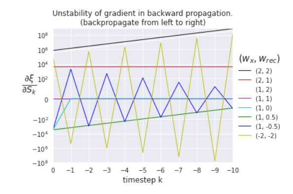
however, We observe that when | wrec | > 1, exploding gradient is observed as illustrated ( wrec =2, wx =2, black line), ( wrec =-2, wx =2, yellow line) and when | wrec | < 1, vanishing gradient is observed as illustrated ( wrec =0.5, wx =1, green line), ( wrec =-0.5, wx =1, dark blue line). When wrec = 1 (illustrated as ( wrec =1, wx =2, red line) and ( wrec =1, wx =1, magenta line), ( wrec =2, wx =2, black line)), gradient stay constant over time and when wrec = 0 (illustrated as ( wrec =0, wx =1, light blue line)), gradient quickly comes to 0.
It is because the gradient of a state Yk between a state m timesteps back ( Yk−m ) can then be written as:
YkYk-m = YkYk-1 …..Yk-m+1Yk-m=wrecm
This is the reason that wrec is less than 1, it tends to 0 as m increases and learning gets stopped since weights cannot significantly change in the backpropagation step. When wrec is negative, gradient changes sign(positive when m even and vice versa )
Step 7: Use Rprop (Resilient Propagation) as an optimization algorithm.
however, you can use the library (if any) for this part Plot the optimization trajectory on the loss surface.
| # Define Resilient prop optimisation functiondef update(train_X, train_Y, W, W_prev_sign, W_del, param_epsilon_p,param_epsilon_n): # Get the gradients by performing forward and backward pass S = forward_states(train_X, W[0], W[1]) grad_out = output_gradient(S[:,-1], train_Y) W_gradients, _ = backward_pass(train_X, S, grad_out, W[1]) W_sign = np.sign(W_gradients) # Sign of new gradient # For each weight parameter, update the Delta (update value)separately for k, _ in enumerate(W): if W_sign[k] == W_prev_sign[k]: W_del[k] *= params_epsilon_p else: W_del[k] *= params_epsilon_n return W_del, W_sign# Perform Rprop optimisation # Hyperparametersparams_epsilon_p = 1.2params_epsilon_n = 0.5 # Set weight parametersW = [-1.5, 2] # [wx, wRec](one is weight that multiplied by input and other is recursive weight)W_del = [0.001, 0.001] # Update values (Delta) for WW_sign = [0, 0] # Previous sign of W list_of_ws = [(W[0], W[1])] # List of weights to plot# Iterate over 500 iterationsfor i in range(500): W_del, W_sign = update( train_X, train_Y, W, W_sign, W_del, params_eta_p, params_eta_n) # Update the weight parameters for k, _ in enumerate(W): W[k] -= W_sign[k] * W_del[k] # Append weights to list for plotting usage list_of_ws.append((W[0], W[1])) print(f’ Final weights are: wx = {W[0]:.4f}, wRec = {W[1]:.4f}’) |
⇒ Final weights are: wx = 1.0014, wRec = 0.9997
Step 8: Plot the loss surface with the weights over the iterations.
| # Define plot functiondef plot_optimisation(list_of_ws, loss_function): ws_1, ws_2 = zip(*list_of_ws) fig = plt.figure(figsize=(10, 4)) # Plot figures axis_1 = fig.add_subplot(1, 2, 1) # Plot overview of loss function ws_1_1, ws_2_1, loss_ws_1 = loss_surface( -3, 3, -3, 3, 100, loss_function) surface_1 = plot_surface(axis_1, ws_1_1, ws_2_1, loss_ws_1 + 1) axis_1.plot(ws_1, ws_2, ‘wo’, markersize=3) axis_1.set_xlim([-3, 3]) axis_1.set_ylim([-3, 3]) axis_2 = fig.add_subplot(1, 2, 2) # Plot zoom of loss function ws_1_2, ws_2_2, loss_ws_2 = loss_surface( 0, 2, 0, 2, 100, loss_function) surface_2 = plot_surface(axis_2, ws_1_2, ws_2_2, loss_ws_2 + 1) axis_2.set_xlim([0, 2]) axis_2.set_ylim([0, 2]) surface_2 = plot_surface(axis_2, ws_1_2, ws_2_2, loss_ws_2) axis_2.plot(ws_1, ws_2, ‘wo’, label=’Rprop iterations’, markersize=3) axis_2.legend() # Display colorbar fig.subplots_adjust(right=0.8) cax = fig.add_axes([0.85, 0.12, 0.03, 0.78]) color_bar = fig.colorbar(surface_1, ticks=np.logspace(0, 8, 9), cax=cax) color_bar.ax.set_ylabel(‘$\\xi$’, fontsize=12) color_bar.set_ticklabels([‘{:.0e}’.format(j) for j in np.logspace(0, 8, 9)]) plt.suptitle(‘Loss surface’, fontsize=12) plt.show() # Plot the optimisationplot_optimisation( list_of_ws, lambda wt1, wt2: loss(forward_states(train_X, wt1, wt2)[:,-1] , train_Y))plt.show() |

Our Linear RNN model is well trained since mean squared error is very low. Yes, it thus counts very well numbers of 1’s in binary sequence and if we round off our output. so, it will be exactly the same as the count. however, Resilient Propagation has worked very well with the given hyperparameter.
Step 9: Predict the test-set data
| print(f’ Final weights are: wx = {W[0]:.4f}, w_rec = {W[1]:.4f}’)print (“Real: \t\t”, testY) y = forward_states(testX, W[0],W[1]) print (“Predicted: \t”,y[:,-1])print(“MSE loss = “,loss(testY, y[:,-1])) |

Conclusion | Linear RNN From Scratch
however, Our Linear RNN is able to predict closely the test-set data.
Written By: Himanshu Kumar Singh
Reviewed By: Rushikesh Lavate
If you are Interested In Machine Learning You Can Check Machine Learning Internship Program
Also Check Other Technical And Non Technical Internship Programs