
What is Linear Regression??
Linear regression is perhaps one of the most well known and well understood algorithms in statistics and machine learning.
Linear regression makes an attempt to model the link between 2 variables by fitting an equation to determine information. One variable into account to be Associate in Nursing informative variable, and therefore the different is take up into account to be a variable
So, this algorithm is basically having a motto to find out the correlation between the various features and this ultimately outputs a prediction of our desired feature and Most Importantly, One may not require any proficient knowledge in statistics to dive deep into this world famous algo “Linear Regression”.
Then We have Hypothesis !!
So, We have our hypothesis as following:
hθ(x) = θ0 + θ1x
Note that this is like the equation of a straight line. We give hθ(x) values for θ0 and θ1 to get our estimated output. So, ultimately we are finding out the optimum values for θ0 and θ1 , when the values of θ0 and θ1 then we can substitute the value of x in the hypothesis, which ultimately results us the desired output value. So that hypothesis is in the form of a straight line and that straight fits our dataset and the output value is of maximum efficiency, On condition that the trained model is optimum.

Costy Func!!
We can measure the accuracy of our hypothesis function by using a cost function. This takes an average (actually a fancier version of an average) of all the results of the hypothesis with inputs from x’s compared to the actual output y’s.

This operation is referred to as the “Squared error function”, or “Mean square error”. The mean is halved (1/2m) as a convenience for the computation of the gradient descent because the by-product term of the sq. operate can eliminate the 1/2 term
Now we have a tendency to square {measure} able to concretely measure the accuracy of our predictor operating against the proper results we’ve got in order that we are able to predict new results we do not have.
If we have a tendency to try and think about it in visual terms, our data set scatters on the x-y plane. we have a tendency to attempt to create a line (define by hθ(x) that passes through this scatter set of the dataset. Our objective is to urge the simplest potential line. The simplest potential line is such that the common square vertical distances of the scattered points from the line are the smallest amount and that hypothesis predicts our prediction. If for the best case, if that line passes through all the points in our dataset then our cost function will be 0 as there is no squared error.
Gradient Descent:
So we’ve got our hypothesis to operate and that we have some way of measure, well it fits into the info currently, we want to estimate the parameters in the hypothesis operate. that is wherever gradient descent comes in.
Imagine that we have a tendency to graph our hypothesis operate supported its fields θ0+θ1 (actually we have a tendency to area unit graphing the value operate as an operation of the parameter estimates). this will be quite confusing; we have a tendency to area unit moving up to a better level of abstraction. we have a tendency to aren’t graphing x and y itself, however, the parameter varies as our hypothesis operates and also the value ensuing from choosing an explicit set of parameters.
We place on the x-axis and θ1 on the y axis, with the value, operate on the vertical z-axis. The points on our graph are the results of the value operate victimization of our hypothesis with those specific alphabetic character parameters.
We will grasp that we’ve succeeded once our value operation is at the terribly bottom of the pits in our graph, i.e. once its price is that the minimum.
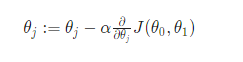
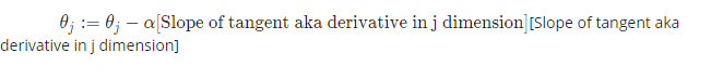
The method we have a tendency to do that is by taking the by-product (the tangential line to operate) of our value function. The slope of the tangent is that the by-product at that time and it’ll provide the North American nation a direction to maneuver towards. We have a tendency to create steps down the value that operate within the direction with the steep descent, and also the size of every step set by the parameter α. that is term the training rate.
The gradient descent algorithm is:
So, we need to run this gradient descent until we get the optimum and much efficient parameters.
thus, this alternatively can be:
So, for Linear Regression:
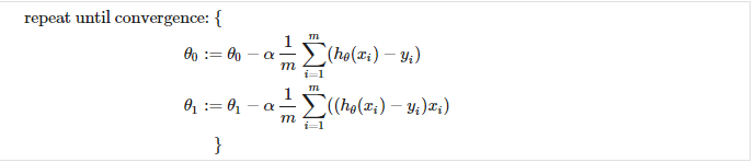
where m is the size of the training set, θ0 a constant that will be changing simultaneously with θ1 and xi , yi are values of the training set.
The point of all this is that if we start with a guess for our hypothesis and then repeatedly apply these gradient descent equations, our hypothesis will become more and more accurate
Summary
So, in this article we have seen the in-depth of linear regression. Linear Regression is a handy tool for a data scientist for solving the rigid business problems and we can also use Deep Learning and Neural Networks for solving the linear regression with much more efficiency.
written by: Naveen Reddy
reviewed by: Krishna Heroor
If you are Interested In Machine Learning You Can Check Machine Learning Internship Program
Also Check Other Technical And Non Technical Internship Programs