Hidden Markov Model | HMM

Hidden Markov Model, Also Abbreviated As HMM, Is A Statistical Model, Which Includes Both Hidden And Observed States. 

https://www.canva.com/design/DAEOTsacoUs/O-MDxmPOLuafOOngWvdv6Q/edit

however, The Data Underlying The Markov Process Is Hidden Or Unknown To The User. thus, Only Observational Data Users Can Know And Monitor. 

https://www.canva.com/design/DAEOastwOR0/UPgHIWL_jPP7Stdhqs9e4g/edit

It Is Important To Note That The Number Of Observable States And The Number Of States In The Hidden Process May Be Different. 

therefore, The Diagram Shows The Observable And Hidden States In The Weather Example. 

https://www.canva.com/design/DAEOa4Aepvw/G2P1IE2n89ncqrZNQK2eoA/edit

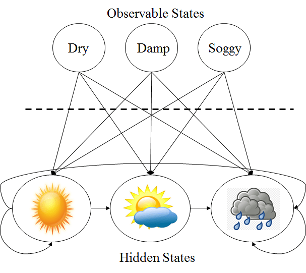
In The Above Diagram It Is Assumed That Hidden States (The True Weather) Are Modelled By Using A Simple First Order Markov Process, And So They Are All Connected To Each Other. 

The Relationship Between The Observable And Hidden States Denote The Probability Of Generating A Specific Observed State Given That The Markov Process Is In A Specific Hidden State. 

It Must Be Clear That All Probabilities “Incoming” An Observable State Will Sum To 1, Since In The Above Example It Would Be The Sum Of Pr(Obs|Cloud), Pr(Obs|Sun), And Pr(Obs|Rain).

HMM Has Two Types of Probabilities: 

1. Transition Probability: thus, Each Transition From Current State To New State Assigned With Probability Value.
2. Emission Probability: also, Each symbol In Each State Assigned With Probability Value.

Example Of HMM:

https://www.canva.com/design/DAEOU9Y03Ro/U6XvVjkPC6NEtfskJjz2wg/edit

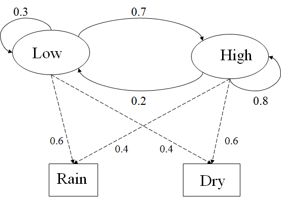
Two states : ‘High’ and ‘Low’ atmospheric pressure.

Two observations : ‘Rain’ and ‘Dry’.

Transition Probability:

P(‘High’|‘High’)=0.8, P(‘High’|‘Low’)=0.7,  P(‘Low’|‘High’)=0.2,  P(‘Low’|‘Low’)=0.3.

Observation probabilities:

P(‘Dry’|‘High’)=0.3, P(‘Rain’|‘High’)=0.4,  P(‘Dry’|‘Low’)=0.4, P(‘Rain’|‘Low’)=0.6. 

Initial probabilities

let’s say 

P(‘High’)=0.6, P(‘Low’)=0.4. 

so, Suppose we want to calculate a probability of a sequence of observations in our example,  {‘Dry’, ’Rain’}.

Consider all possible hidden state sequences:

P({‘Dry’,’Rain’} ) = P({‘Dry’,’Rain’}, {‘High’,’High’}) + P({‘Dry’,’Rain’}, {‘High’,’Low’}) + P({‘Dry’,’Rain’}, {‘Low’,’High’}) +  P({‘Dry’,’Rain’}, {‘Low’,’Low’}) 

where first term is :

P({‘Dry’,’Rain’} , {‘Low’,’Low’})=

P({‘Dry’,’Rain’} | {‘Low’,’Low’})  P({‘Low’,’Low’}) =

P(‘Dry’|’Low’)P(‘Rain’|’Low’) P(‘Low’)P(‘Low’|’Low)= 0.4*0.4*0.6*0.4*0.3

Shorthand Notation Of HMM [λ = (A,B,π)]

Other Notations Are Stated Below

• A = Transition Probabilities Of States 
• B = Probability Matrix Of Observation
• O = Sequence Of Observation 
• π = Initial State Distribution 
• s = Sequence Of States 
• N = Total Number Of states 
• M = Total Number Of Observations
• Q = Discrete States Of The Markov process 
• T = Length Of The Observation Sequence
• V = Finite Set Of Observations Symbol Per States 
• x_k = Hidden State
• z_k = Observation

Three Basic Problems in Hidden Markov Model:

1. In The “Evaluation” Problem, thus, The Known Model And Sequence Of Observation Used To Compute The Likelihood Of An Observation Sequence. 

2. In The “Decoding” Problem, The Known Model And Generated Observed Sequence Used To Obtain The Most Likely Sequence Of Hidden States. These two issues often related with pattern recognition.

3. In The Learning Problem, so The Given Some Training Observation Sequences And General Structure Of HMM (x_k, z_k), Computes HMM Parameters λ=(A,B,π) That Best Fit Training Data.

Evaluation:

Consider The Example, We Have A “Winter” Model And A “Summer” Model For The Seaweed Since Behavior Is Likely To Be Different From Season To Season Then To Determine The Season Based On A Sequence Of Dampness Observations.  

https://www.canva.com/design/DAEOb25YaMY/elLO6YXOt48TetP2mc8Sqw/edit

in order To solve The Problem Of Evaluation Forward, Algorithm Used To Calculate The Probability Of An Observation Sequence With The Help Of A Known HMM Model.

Decoding:

Consider The Example Of The Weather And The Seaweed; A Blind Hermit Can Only Sense The Seaweed State But Needs To Know The Weather.  

To solve The Problem Of Decoding, so, Viterbi Algorithm Used To Determine The Most Probable Sequence Of Hidden States Given Sequence Of Observations And A HMM Model.

Learning:

Correct Selection Of Observation Sequence From Known Set, thus To Represent A Set Of Hidden States And Fit The Most Probable HMM Model Is The Hardest Problem Associated With HMM.

in order To Solve The Problem Of Learning, Baum-Welch Expectation-Maximization (EM) Algorithm Used To Identify Optimal Parameters Of the HMM Model.

Pros:

1. It has a Robust Statistical Foundation
2. Can also Handle Inputs Of Variable Length
3. It Can Be Combined Into Libraries

Cons:

1. It also Has A Huge Number Of Unstructured Factors.
2. thus, it’s Unable To Express Dependencies Between Hidden States.

Applications of Hidden Markov Model:

HMM model is well known for their application in Reinforcement learning and Pattern recognition such as,

1. Speech
2. Text or handwriting Processing
3. Part of speech tagging
4. Gesture Classification
5. Bioinformatics
6. Vehicle Trajectory Projection

Conclusion

In This Article, We Have Learned About the Hidden Markov Model. so, The Concept Of HMM Easily Explained With Simple Example. There Are Three Fundamental Issues That Must Be Solved Before Using HMM. We Have Also Discussed The Types Of Probabilities, Pros, Cons And Its Applications.

Written By: Preeti Bamane

Reviewed By: Rushikesh Lavate

If you are Interested In Machine Learning You Can Check Machine Learning Internship Program
Also Check Other Technical And Non Technical Internship Programs