#Disabling Weight Training
for layer in vgg.layers:
layer.trainable = F
Transfer learning, the name itself depicts the transfer of knowledge from one to another. Likewise, in Transfer learning, we use a pre-trained model and add some more layers to the pre-trained model to generate a new Model to save computational power and processing time.
Let’s take deep dive into the brief concept about Transfer learning as a whole.
Transfer learning is also a problem solution in deep learning that uses pre-trained datasets to find an efficient solution for the required prediction, feature extraction, and fine-tuning.
Why to use Transfer Learning?
The main problem faced by a data scientist is the time required for training datasets. What if? though You use a pre-trained model for building your model. It might sound unrealistic for the first time but, yes it’s possible with the help of some pre-trained model provided by Keras. Hence, Depending on which type of model you want to train, you can choose the pre-trained Keras model.
When does Transfer learning make sense?
- When your dataset contains very little data to train your model to give high accuracy results.
Suppose, ‘A’ is my pre-trained model from Keras whereas ‘B’ is the dataset which we’ll be using for prediction.
- When A and B have the same inputs.
For example, A contains a dataset of images containing different diseases in crops and you are feeding B with an animal’s dataset then, in this case, the model won’t work.
Assume another instance, if A contains a dataset of images containing different diseases in crops and B contains a dataset of healthy crops and you want to predict the output for healthy crops, in this case, your model won’t give the correct result.
So, A and B should contain related data to get accurate results.
- The number of data in A should be more than B.
- Low-level features from A can be helpful also for learning B.
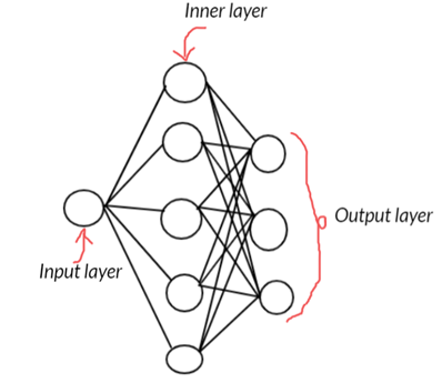
Flow-chart of model building in Transfer Learning

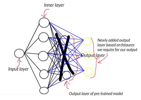
Freezing the layers means to convert the trainable layers to non-trainable. By doing this, when we will train the newly added layers, these pre-trained layers won’t get trained again, thus saving computational process and time.
however, Unfreezing the layers means to convert back the frozen layers to trainable ones.
Illustration on TL
Suppose, this is my pre-trained model
Now, take an example that your pre-trained model contains a dataset for a car and you want to build a model that predicts whether the image is of a truck or not. But some layers in the pre-trained model of cars are helpful to train the model for some truck’s feature like mirror, color, graphics, door, wheels, etc. so we’ll use these common layers and remove the layers which are not related to trucks and add some more layers that will specify other features of the truck. This is the way how Transfer Learning works.
The figure below depicts how we can remove the output layer from the pre-trained model and then add the required features in the output layer.
Let’s have a brief on some important pre-trained Keras Model:
- Xception:
Size: 88MB
Top-5 Accuracy: 0.945
Parameters: 22,910,480
Depth: 126
- VGG16:
Size: 528 MB
Top-5 Accuracy: 0.901
Parameters: 138,357,544
Depth: 23
- VGG19:
Size: 549 MB
Top-5 Accuracy: 0.900
Parameters: 143,667,240
Depth: 26
- ResNet50:
Size: 98 MB
Top-5 Accuracy: 0.921
Parameters: 25,636,712
Depth: –
- ResNet101:
Size: 171 MB
Top-5 Accuracy: 0.928
Parameters: 44,707,176
Depth: –
- ResNet152:
Size: 232 MB
Top-5 Accuracy: 0.931
Parameters: 60,419,944
Depth: –
For more models, refer: https://keras.io/api/applications/
Hands-on: how TL works?
Problem Statement:
Model to detect any symptoms of pest/disease of crop based on image analysis of the leaves. (Plants covered: Pepper, Potato, Tomato)
In this model, we’ll be using the VGG16 model for Transfer learning.
First, we’ll be importing libraries,
Lamba-> Activation function
Dense->Type of layer in DNN
VGG16->Pre-trained Keras model
Model-> This function will help us to build the model
#For generating neural network / nodes
from keras.layers import Input, Lambda, Dense, Flatten
#For Initializing the model
from keras.models import Model
#For defining the architecture Employed
from keras.applications.vgg16 import VGG16
from keras.applications.vgg16 import preprocess_input
#For pre-processing and Image Augmentation
from keras.preprocessing import image
from keras.preprocessing.image import ImageDataGenerator
#For enabling Sequential Layer
from keras.models import Sequential
#For files retrieval and path
from glob import glob
#For visualization
import matplotlib.pyplot as plt
Before importing the model, we’ll define the input image size to 224 x 224.
Then, we’ll import our train and validation dataset. so, In this code, I’ve uploaded my dataset separated as train and validation through Google drive.
#Pre-defining the Image Size
IMAGE_SIZE = [224, 224]
#Mounting Google drive path
train_path = ‘/content/drive/My Drive/Data-Set/Train’
valid_path = ‘/content/drive/My Drive/Data-Set/Test/Test’
Now, we’ll be importing the VGG16 dataset and then freezing the layers of VGG16.
# add preprocessing layer to the front of VGG
vgg = VGG16(input_shape=IMAGE_SIZE + [3], weights=’imagenet’, include_top=False)alse
Here, we will create a Dense layer for output and then build our model.
#Variable for storing number of files
folders = glob(‘/content/drive/My Drive/Data-Set/Test/Test/*’)
print(len(folders))
# our layers – you can add more if you want
x = Flatten()(vgg.output)
# x = Dense(1000, activation=’relu’)(x)
prediction = Dense(len(folders), activation=’softmax’)(x)
# create a model object
model = Model(inputs=vgg.input, outputs=prediction)
# view the structure of the model
model.summary()
Now, we’ll compile the model, which includes defining the loss function, optimizer.
Then, we’ll augment the data. so, The main reason behind Data Augmentation is to reduce Overfitting. Data Augmentation helps us to increase data in our dataset by modifying the existing data by zooming-in/ zooming-out/ rotating the images/ mirror image and so on.
# Defining Loss function and optimizer to be used
model.compile(
loss=’categorical_crossentropy’,
optimizer=’adam’,
metrics=[‘accuracy’]
)
# Data Augmentation
from keras.preprocessing.image import ImageDataGenerator
train_datagen = ImageDataGenerator(rescale = 1./255,
epochs=5,
steps_per_epoch=len(training_set),
validation_steps=len(test_set)
)
Last step is to save the Model
import tensorflow as tf
from keras.models import load_model
model.save(‘Transfer_Learning_01.h5’)
The most important thing to keep in mind: We have used the VGG16 model in this code, if you want to use any other pre-trained model according to your computational power and device few minor changes need to be considered in above given code.
Hence, now you have understood the basics of Transfer Learning and will be able to apply your knowledge in real life problems.
Keep learning! Keep sharing!
shear_range = 0.2,
zoom_range = 0.2,
horizontal_flip = True)
Then, we’ll be generating training and test data.
# Uniforming the datagen
test_datagen = ImageDataGenerator(rescale = 1./255)
# Training Set
training_set = train_datagen.flow_from_directory(train_path,
target_size = (224, 224),
batch_size = 32,
class_mode = ‘categorical’)
# Test Set
test_set = test_datagen.flow_from_directory(valid_path,
target_size = (224, 224),
batch_size = 32,
class_mode = ‘categorical’)
Now, we’ll finally apply the fit generator method to get the results.
# fit the model
r = model.fit_generator(
training_set,
validation_data=test_set,
Last step is to save the Model.
import tensorflow as tf
from keras.models import load_model
model.save(‘Transfer_Learning_01.h5’)
Conclusion
The most important thing to keep in mind: We have used the VGG16 model in this code, if you want to use any other pre-trained model according to your computational power and device few minor changes need to be considered in above given code.
Hope, now you have understood the basics of Transfer Learning and will be able to apply your knowledge in real life problems.
Keep learning! Keep sharing!
Written by: Ketki Kinkar
Reviewed By: Savya Sachi
If you are Interested In Machine Learning You Can Check Machine Learning Internship Program
Also Check Other Technical And Non Technical Internship Programs