
Gradient Descent is an optimization Concept in the ML & deep learning process which helps us minimize the cost function by learning the weights of the model such that it fits the training data well. Its Minimize the errors algorithm:
Error= (Actual value -predicted value)
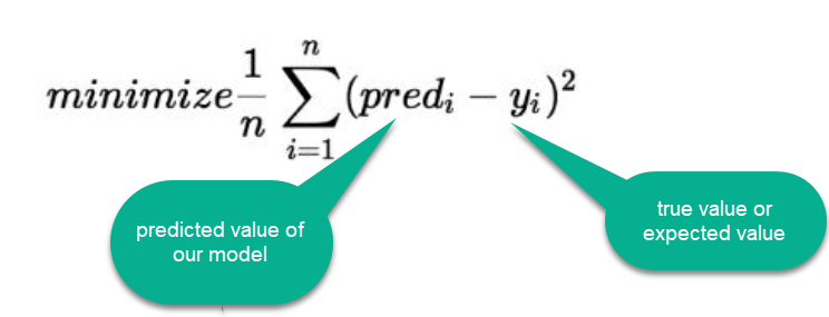
Cost function
Types of cost functions
- Mean Squared Error
- Root Mean Squared Error
- Mean Absolute Error
In statistics, machine learning and other data science fields we optimize a lot of stuff.
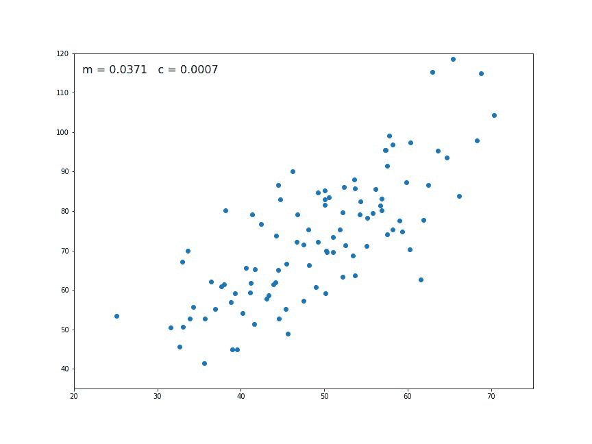
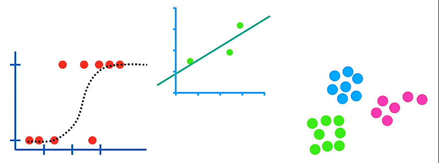
When we fit a line with linear regression, we optimize the intercepts and slope.
y = mx + c
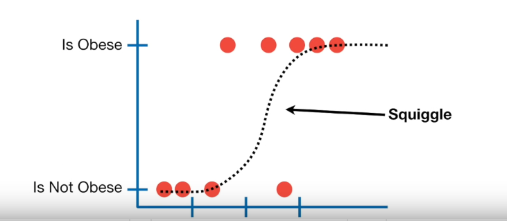
When we use logistic regression, we optimize a squiggle
When we deal with T-SHE we optimize clusters.

These are the just few examples we optimize, there are tons more.
The great thing is that GD can optimize all these things and much more.
Gradient = rate of inclination or going declination of a slope (how steep a slope is and in which direction it is ) of a function at some point.
Descent = an act of moving downwards.
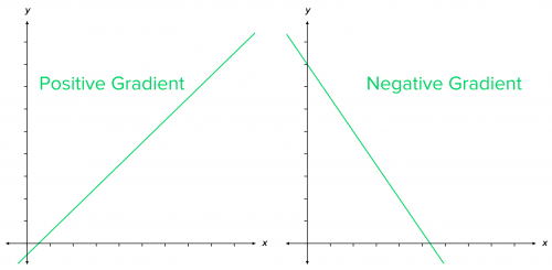
Simple way to memorize:
- line going up as we move right → positive slope, gradient
- line going down as we move right → negative slope, gradient
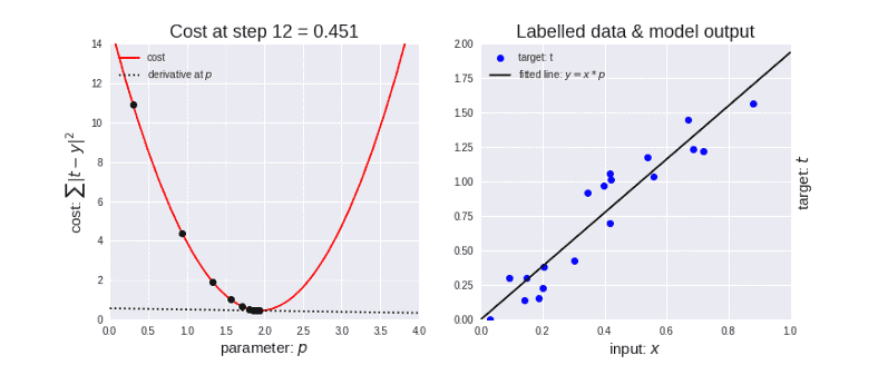
At the start, the parameter values of the hypothesis are randomly initialized (can be 0).
Then, Gradient Descent iteratively (one step at a time) adjusts the parameters and gradually finds the best values for them by minimizing the cost.
In this case we’ll use it to find the parameters m and c of the linear regression model.
m = slope of a line that we just learned about.
c = bias: where the line crosses the Y axis.
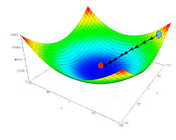
Imagine a person at the top of a mountain who wants to get to the bottom of the valley below the mountain through the fog (he cannot see clearly ahead and only can look around the point he’s standing at).
He goes down and takes large steps when the inclination is high and small steps when the inclination is low.
He decides his next position based on his current position and stops when he gets to the bottom of the valley which was the minimum point of the valley.

Gradient descent action
Now, think of the valley as a cost function.
The objective of GD is to minimise the cost function (by updating its parameter values). In this case the minimum value would be 0.
MSE= 1ny-y2
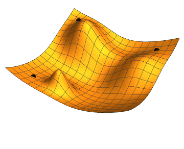
How its looks like:
J is the cost function, plotted along it’s parameter values. Notice the crests and troughs.
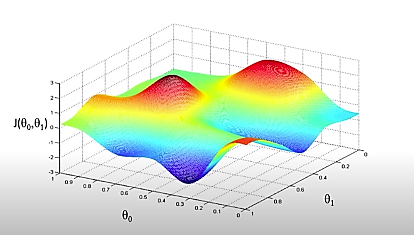
How we navigate the cost function via GD:
Gradient Descent Types
- Batch Gradient Descent: processes all the training data for each iteration. For large amounts of training data, batch gradient computationally hard requires a lot of time and processing speed to do this task. So, for large number of training data we prefer to use mini or stochastic method.
- Stochastic Gradient Descent: This GD processes one training data per iteration. Only single training data is processed at a time and the next one being updated after completion of one. It can process large training data. only one example which can be additional overhead for the system as the number of iterations will be quite large.
- Mini Batch gradient descent: This which works faster than both batch gradient descent and stochastic gradient descent. Here b examples where b<m are processed per iteration. So even if the number of training examples is large, it is processed in batches of b training examples in one go. Thus, it works for larger training examples and that too with lesser number of iterations.
Importance of Learning rate:
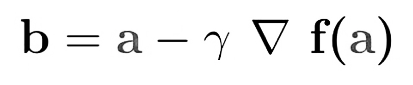
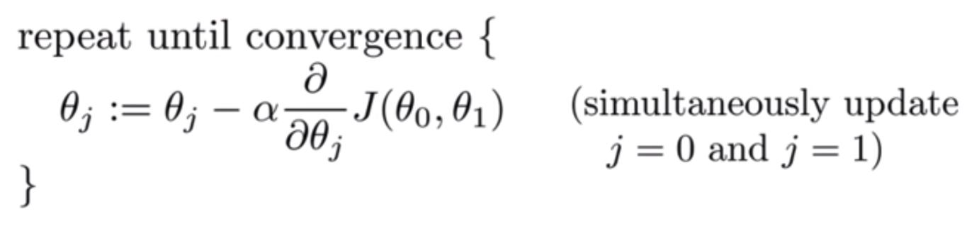
The equation above describes what gradient descent does: b is the next position of our climber, while a represents his current position. The minus sign refers to the minimization part. The gamma in the middle is a waiting factor and the gradient term (Δf(a)) is simply the direction of the steepest descent.
How big the steps are gradient descent takes into the direction of the local minimum are determined by the learning rate, which figures out how fast or slow we will move towards the optimal weights.
For gradient descent to reach the local minimum we must set the learning rate to an appropriate value, which is neither too low nor too high. This is important because if the steps it takes are too big, it may not reach the local minimum because it bounces back and forth between the convex function of gradient descent (see left image below).
If we set the learning rate to a very small value, gradient descent will eventually reach the local minimum but that may take a while (see the below image).

So, the learning rate should never be too high or too low for this reason. You can check if your- learning rate is doing well by plotting it on a graph.
Conclusion
So that was all about gradient descent briefly….I hope you got an idea of how it works
Article by: Sachin Dubey
If you are Interested In Machine Learning You Can Check Machine Learning Internship Program
Also Check Other Technical And Non Technical Internship Programs