

In this article, we will learn about Grad-CAM
- Introduction
- How does it work?
- Implementation
Introduction:
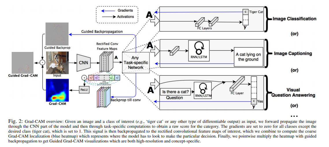
Grad-CAM (Gradient-weighted Class Activation Mapping) is a popular technique for visualizing where a convolutional neural network model is looking. It is class-specific, i.e. it produces a separate visualization for each input class i.e. image.
There are other methods like CAM to visualize CNN, but it has drawbacks that it requires feature maps to directly precede the softmax layers, so it can be applied to a particular kind of CNN architectures that perform prediction immediately after global average pooling over convolutional maps.
In short, the CAM architecture requirement is convolution feature maps → global average pooling →softmax layer. One can see such architectures may achieve inferior accuracies compared to general networks on some tasks or simply be inapplicable to new tasks.
How Grad-CAM works?
In CNN, we can also take images and operate it over convolutional layers with the help of filters. So we actually take out the spatial information of the images through convolutional layers and the last convolutional layer is responsible for the features on which CNN predicts the output.
Furthermore, CNN loses its spatial information in fully-connected layers, so the last convolutional layer has the best compromise between high-level semantics and detailed spatial information.
So first we train our CNN model on the train set for the specific task. During training, appropriate weight and bias values are assigned to the model through forward-pass and backward-pass. so, we find a class discriminative localization map that has the same size as our input image. thus, It contains information for each neuron responsible for the decision of the model.
To calculate, class discriminative localization map, we find out the average gradient of output ycbefore softmax with respect to the last convolutional layer Aijk. This average is specifically called the global average pooled. We then find out heat-map by applying ReLu to a weighted combination of activation maps as given in the steps.
In short, it involves three steps:
1. Compute gradient
Compute the gradient of output yc before softmax with respect to last convolution activation layer Aijk
Gradient =ycAijk
2. Average alpha (ck) by averaging the gradients
ck =1ZijycAijk

3. Calculate the final Heat Map:
We perform a weighted combination of activation maps and follow it by ReLU. thus, Notice that this results in heatmap to be the same size as the convolutional feature maps

Implementation:
We will also be training CNN (VGG16 model) to classify the dog breed. so, We will be using data from Kaggle (https://www.kaggle.com/samcrochet/p29crosspuredogs) containing 15 breeds of dog.
Here is the original Grad-CAM article: https://arxiv.org/pdf/1610.02391.pdf
Here is the implementation of Grad-CAM with the VGG16 model: https://colab.research.google.com/drive/1X4Ttgbchr74Tm7AO0I-P4Rz-xGJ0w1Eo?usp=sharing
Part-1: Training CNN
Step-1: Download the pre-trained VGG16 model.
Step-2: Modify the final fully connected layer to accommodate 15 classes
Step-3: Finetune the model to classify the given dataset of 15 dog breeds
Part-2: Implementing Grad-CAM
Step-4: We need to identify the last convolutional layer and subsequent classifier layer name. In the case of VGG16, the last convolution layer is block5_Convolution layer 3. It will change according to the model, but the crux is to identify the last convolution layer. It is to identify the subsequent classifier layer name i.e. all the layers after the last convolution layer. This layer will be used to find the gradient i.e. ycAijk using the chain rule. Here yc is output before softmax and Aijk is the last convolutional layer
last_convolutional_layer_name = “block5_conv3”
classifier_layers = [ “block5_pool”, “flatten”, “fc1”, “fc2”, “dense”,]
Step-6: Make a function to preprocess the image
def get_img_array(img_path, size):
img = keras.preprocessing.image.load_img(img_path, target_size=size)
array = keras.preprocessing.image.img_to_array(img)
array = np.expand_dims(array, axis=0)
return array
Step-7: Make a heat-Map function
def make_gradcam_heatmap( img_array, model, last_convolution_layer_name, classifier_layers):
# Create a last_convolutional_layer_model to map the input image to the activations of the last convolutional layer
last_convolutional_layer = model.get_layer(last_convolutional_layer_name)
last_convolutional_layer_model = keras.Model(model.inputs,last_convolutional_layer.output)
# Create a classifier_model to map the activations of the last convolutional layer to the final class predictions
classifier_input = keras.Input(shape=last_convolutional_layer.output.shape[1:])
x = classifier_input
for layer_name in classifier_layers:
x = model.get_layer(lclassifier_layers)(x)
classifier_model = keras.Model(classifier_input, x)
# Compute the gradient of the top predicted class for our input image with respect to the activations of the last convolutional layer
with tf.GradientTape() as tape:
# Compute activations of the last convolutional layer and make the tape watch it
last_convolutional_layer_output = last_convolutional_layer_model(img_array)
tape.watch(last_convolutional_layer_output)
# Compute class predictions
preds = classifier_model(last_convolutional_layer_output)
top_pred_index = tf.argmax(preds[0])
top_class_channel = preds[:, top_pred_index]
# grads is the gradient of the top predicted class with regard to the output feature map of the last convolutional layer
grads = tape.gradient(top_class_channel, last_convolutional_layer_output)
# pooled_grad is a vector where each entry is the mean intensity of the gradient over a specific feature map channel
pooled_grads = tf.reduce_mean(grads, axis=(0, 1, 2))
# Multiply each channel in the feature map array by “how important this channel is” with regard to the top predicted class
last_convolutional_layer_output = last_convolutional_layer_output.numpy()[0]
pooled_grads = pooled_grads.numpy()
for i in range(pooled_grads.shape[-1]):
last_convolutional_layer_output[:, :, i] *= pooled_grads[i]
# The channel-wise mean of the resulting feature map is our heatmap of class activation
heatmap = np.mean(last_convolutional_layer_output, axis=-1)
# Normalize the heatmap between 0 & 1 for visualization purposes.
heatmap = np.maximum(heatmap, 0) / np.max(heatmap)
return heatmap
Conclusion:
We can thus visualize the feature selection of CNN with the help of Grad-CAM. Moreover, interpretability of AI is most tasks because when today’s intelligent systems fail, they fail spectacularly disgracefully without warning or explanation, leaving a user staring at an incoherent output, wondering why.
Have a nice day! Bye
written by: Himanshu Kumar Singh
reviewed by: Rushikesh Lavate
If you are Interested In Machine Learning You Can Check Machine Learning Internship Program
Also Check Other Technical And Non Technical Internship Programs