Excelling at Machine Learning is a cakewalk. Most of the beginners start with learning linear regression and then take a step forward to logistic regression, But does that solve our purpose?! Of Course not! Because you can make out more rather than using regression.
There is a saying Once said, excelling in machine learning is not just by grasping knowledge and being proficient with machine learning algorithms, It’s all about using the correct ML algorithm for the correct scenario. As an analogy, consider ‘Regression’ as an arm capable of slicing and dicing information with efficiency, however incapable of managing extremely complicated information.
On the contrary, ‘Support Vector Machine’ is sort of a sharp bow and it works on smaller datasets, however, on the complicated ones, it may be abundant stronger and powerful in building machine learning models. You will get to know all the things in a detailed manner, Once if you complete this blog. Till then stay thrilled 😉
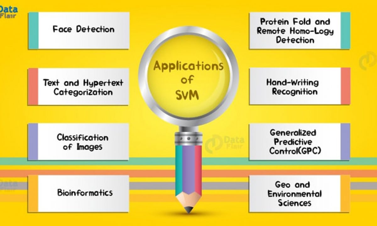
Use Cases of SVMs:
What is a Support Vector Machine?
In machine learning, support vector machines (SVMs, also support vector networks) are supervised learning models with associated learning algorithms that analyze data used for classification and regression analysis. Given a set of training examples, each marked as belonging to one or the other of two categories, an SVM training algorithm builds a model that assigns new examples to one category or the other, making it a non-probabilistic binary linear classifier. So we can check out the use of SVMs in a trend ranging through years!!
(Source: Google Trends)
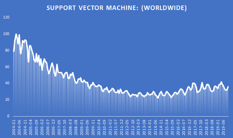
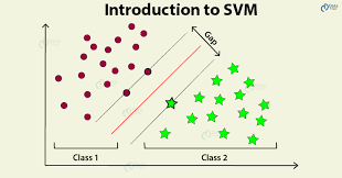
So these SVMs became flavor to many and these are used widely across different parts of the earth. However, it is mostly used in classification problems. In the SVM algorithm, we plot each data item as a point in n-dimensional space (where n is number of features you have) with the value of each feature being the value of a particular coordinate. WAIT, This is not yet done!!! Bare with me for a couple of slides to know more about features.
Grab Some Distinction B/W SVMs and Logistic Regression!!!

So this makes sense right?! As we can observe the main and foremost important contrast between the Cost Functions. Furthermore, convention dictates that we regularize using a factor C, instead of λ, like so.This is admiring multiplying the equation by C = 1/λ , and therefore ends up in a similar value once optimized.
Now, after we would like to regularize a lot of (that is, cut back overfitting), we tend to decrease C, and after we would like to regularize less (that is, cut back underfitting), we tend to increase C.
Finally, note that the hypothesis of the Support Vector Machine is not interpreted as the probability of y being 1 or 0 (as it is for the hypothesis of logistic regression). Instead, it outputs either 1 or 0. (In technical terms, it is a discriminant function.)
working of SVMs
A useful way to think about Support Vector Machines is to think of them as Large Margin Classifiers.
If y=1, we want xΘT≥ 1 (not just ≥0)
If y=0, we want xΘT≤ 1 (not just <0)
Now when we set our constant C to a very large value (e.g. 100,000), our optimizing function will constrain Θ such that the equation A (the summation of the cost of each example) equals 0. We impose the following constraints on Θ:
XΘT≥ 1 if y = 1 and XΘT≤ −1 if y=0
If C is very large, we must choose Θ parameters such that it reduces our cost function.
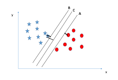
Recall the choice boundary from supplying regression (the line separating the positive and negative examples). In SVMs, the choice boundary has the special property that it’s as secluded as doable from each the positive and also the negative examples. The distance of the choice boundary to the closest example is named the margin.
Since SVMs maximize this margin, it’s usually known as an oversized Margin Classifier. The SVM can separate the negative and positive examples by an oversized margin. This giant margin is barely achieved once C is extremely large. Data is linearly divisible once a line will separate the positive and negative examples.
If we’ve got outlier examples that we do not need to have an effect on the choice boundary, then we are able to cut back C. Increasing and decreasing C is comparable to severely decreasing and increasing λ, and might change our call boundary.
Kernels:
Kernels allow us to make complex, non-linear classifiers using Support Vector Machines.
Given x, compute new feature depending on proximity to landmarks l(1),l(2),l(3)
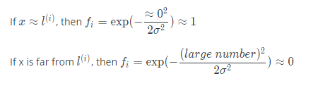
This “similarity” function is called a Gaussian Kernel. It is a specific example of a kernel.
The similarity function can also be written as follows:

f i = similarity(x,l(i))=
if x and the landmark are close, then the similarity will be close to 1, and if x and the landmark are far away from each other, the similarity will be close to 0.
One way to get the landmarks is to put them in the exact same locations as all the training examples. This gives us m landmarks, with one landmark per training example.
f1= similarity(x,l(1)) , f2= similarity(x,l(2)) , f3= similarity(x,l(3)) and so on
And now using these features , we concatenate into example x(i)
Now to get the parameters Θ we can use the SVM minimization algorithm but with f(i) substituted in for x(i)
Using SVMs:
In practical application, the choices you do need to make are:
- Choice of parameter C
- Choice of kernel (similarity function)
- No kernel (“linear” kernel) — gives standard linear classifier
- Choose when n is large and when m is small
- Choose when n is small and m is large
Note: do perform feature scaling before using the Gaussian Kernel.
But When to use SVMs and Logistic Regression?
If n is giant (relative to m), then use logistic regression, or SVM while not a kernel (the “linear kernel”) If n is tiny and m is intermediate, then use SVM with a Gaussian Kernel If n is tiny and m is giant, then manually create/add additional options, then use logistic regression or SVM while not a kernel.
In the 1st case, we do not have enough examples to want an advanced polynomial hypothesis. Within the second example, we’ve got enough examples that we tend to have a fancy non-linear hypothesis. Within the last case, we would like to extend our options so that logistical regression becomes applicable.
Summary And Farewell:
So, We have Explored the math behind SVMs and I hope this blog post helped in understanding SVMs.
written by: Naveen Reddy
reviewed by: Krishna Heroor
If you are Interested In Machine Learning You Can Check Machine Learning Internship Program
Also Check Other Technical And Non Technical Internship Programs