

Optimization is a mathematical concept which operates in a constrained environment to maximize or minimize an objective function, which has higher dimension complex problems. For instance, if a company’s sales prices are decided by market forces of competition, they would have to minimize their cost function, in order to maximize their profit surplus. therefore, This would require them to allocate their limited resources to channels which satisfy their objective of minimization of cost (the constraint).
Gradient descent is an iterative method of optimization to find the minimum of a cost function. Imagine trekking a mountain valley, gradient descent is analogous to travelling towards the downslope of that mountain, such that converging at its bottom-most point, is our objective. since In Machine Learning(ML), cost function is defined as the average of all the errors between the actual values and those predicted by any ML model at different data points.
Error = |Actual value(Y) – predicted value(f(x))|.
Cost functions are classified into three categories:
- Mean absolute error (MAE).
- Mean square error (MSE).
- Root Mean Squared error (RMSE).
The Root Mean Squared Error(RMSE) Cost function, J() = i=1ny(i) -f(x(i))2 N
N: number of data points
however, The cost function is a measure of performance of any ML model and inadvertently follows a convex upwards parabolic function, such that it has one global minima (with caveats). Thus, the objective of any MLmodel is to minimize this cost function.
Objective: min J(0 ,1)
The Mathematics:
Consider a Cost function: y=(x-8)2, Which can be plotted as:
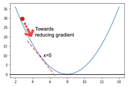
Graphically, it can thus be observed that the minima of this function would be at x=8. But for a deeper understanding of the concept, we shall proceed with the numerical iterative method obtaining minima through gradient descent.
The basic formula of Gradient descent is:
1=0 – J(0)
Where,
0: Initial abscissa value
1: Subsequent abscissa value
: Learning rate.
This is the value of step size we assign to the gradient of the cost function. A larger value would result in a lesser number of training epochs but with a risk of over-shooting the minima and hence, a suboptimal solution whereas a smaller value would result in slower convergence with a large number of epochs coupled with a risk of the process getting stuck.
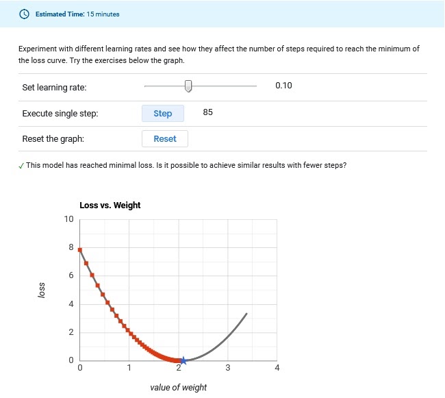
Figure-1: Too Low ,Convergence Too Slow 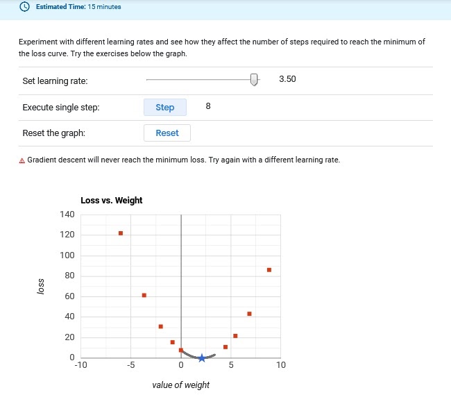
Figure-2: Too High, Doesn’t Converge.
Learning rate optimization
Derivative or slope of function at a particular point.
J(0) : Cost function. Provides direction for gradient descent.
This iterative process continues till the value of cost function converges to its minimum value.
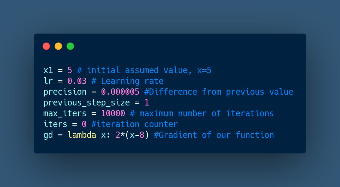
In our given cost function, y=(x-8)2 , we thus assume the initial value of x0 as 5 and as 0.3, such that:
Initial equation:
X1 = X0 – J(X0)
X0= 5
= 0.03
J(X0) = 2(X0-8) = 2(5-8)
Iteration 1:
X1 = 5 – 0.032(5-8)
X1 = 5.18
Iteration 2:
X2 = 5.18 – 0.032(5.18-8)
X2 = 5.3492
In this way, we observe that the value of X is converging towards 8, albeit slowly, where the cost function is attaining its minimum value, thus satisfying our objective.
 Gradient descent in python:
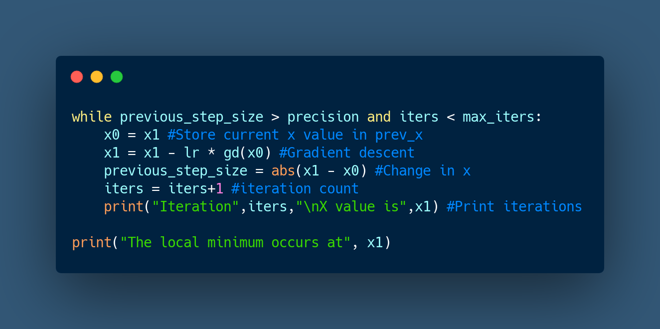
Output:

Hence, the output after 171 iterations, gives the value of x at which global minima for the given function occurs as 7.9999 as compared to the actual value, which was 8.
Conclusion
Summing up, Gradient descent is an optimization tool for a machine learning or a deep learning model so as to reduce the error between the values predicted by the model and the actual values. It involves the concept of differential calculus whereby the cost function moves iteratively towards the direction of minimum gradient, henceforth converging towards a global minima of the respective cost function.
Reviewed By: Vikas Bhardwaj