
Understanding The Mathematics And Computing Logic Behind These Ideas Is Supreme In Building Powerful Recommender System.
Suppose: It is a Friday night and you have had a long week at work or classes – or possibly both. You are looking forward to relaxing with a good movie and some delicious food. You switch over to your preferred streaming service – let’s say Netflix, and immediately attacked with a variety of options.
If a decisive individual or mentally exhausted, this process might be a breeze for you. However, if you are anything like me, then making choices about movies or shows to watch can be difficult. Alternatively, You stare at that screen and scroll endlessly through Netflix’s interface and become increasingly unsettled.
To make matters worse, your stomach complains louder by the minute so you decide to Deliver food. Yet again you faced an irritating amount of varieties. This Friday night has been far from ideal – chaotic end to a stressful week.
Lucky for us, the Recommender System industry is akin to spawning grounds of innovation and problem-solving.
Recommender systems & Types
Recommender System save people like us from the aggravating process of decision making – at least for the not so crucial aspects of life. by doing the work for us. They provide recommendations on what to watch, listen to. or eat based on an integration of both complex and simple algorithms.
unlike the general public who get away with only enjoying the fruits of our labor!
The most commonly used Recommender System are:
1. Content-based recommendations.
2. Collaborative Filtering.
In this post, we will be discussing the second option. For the other one , go through our website Blogs.
Collaborative Filtering:
A collaborative filtering-based Recommender system observes users and understands the models behind their usual choices and maps these learnings with equations to provide support – much like how top-notch customer service from waiters at a well-frequented restaurant provides you with personalized food options.
Consider a system that provides movie recommendations. You sign up for a new streaming service and in the initial days, you provide valuable information to the algorithm by making selections on your own. You may also choose to follow your friends and their customised playlists. Meanwhile, the system maps all this information to the algorithm and starts showing you what you might like to watch. The system doesn’t pay any attention to the actual content of the choices you make, rather it relies entirely on the pattern of your choices, and those of users like you.
There are two basic approaches to this problem:
1. User-based
2. Item-based
Imagine a matrix(technically called utility matrix) of dimensions m x n, with ui users and vj movies (or items in general) – i and j ranging from 1 to m and n respectively. The cells of this matrix represent the association of a user with a movie. That is, the cell rij represents the rating for movie j given by user i.
This matrix already filled in with ratings, i.e. user opinions, either explicitly or implicitly. Explicit rating is when the user provides direct feedback for a movie, for example rating a movie out of 5 stars. Implicit rating – obtained indirectly by tracking the user’s views, page clicks, past choices etc.
For the user-based approach, we aim to predict the target user’s rating for a movie that they haven’t yet watched by measuring the similarity between the target user and the other users. The process is as follows:
Similarity between target & Other user
1. Calculate similarities between the target user and the others
2. Select the top n similar users
3. Calculate the weighted average of the ratings from these n users with similarities as the weights.

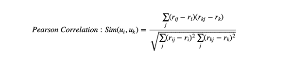
Here we are finding the similarities between the users i and k
This will give us a rating value which then used to provide recommendations. To calculate the similarities, we make use of either of the following two equations,

Ironically, in the pursuit of simplifying the choices in our lives, we face more and more as we go deeper into the logic behind these systems.
Let’s look at an example:
Here we have five different users, with user E being the target user and six different movies.
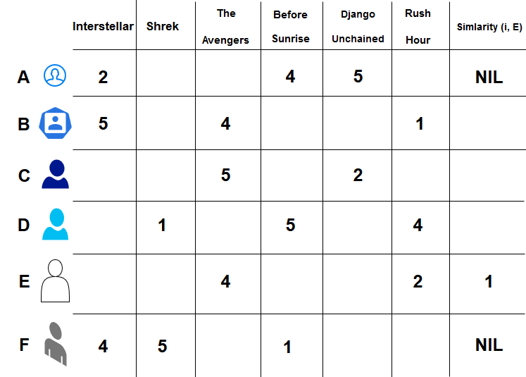
Since there are no common ratings between E and A, and E and F, the similarity values for those two users are NIL.
Similar calculations done using the Pearson Coefficient and provided in the last column.

Now that we have the similarities between the users, we can make predictions on the rating that the target user is likely to give to the unwatched movies and recommend these movies accordingly. (predictions are in red)
The main issue with the user-based approach is the differences between user preferences and the possibility of changes to the same as well.
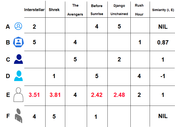
follow the item-based approach
Here we relate items together by stating that two items are similar when they receive similar ratings from the same user. As with the previous method, do a similar calculation using the Pearson coefficient. The only difference is that we make predictions considering a movie (or item) rather than a user. After obtaining the similarities, we predict the user-item pair values non-filled ones.
The biggest drawback of both methods is the possibility of a lack of data. Users seldom leave ratings for the movies they watch, and even if they do, the ratings aren’t always reliable. This results in the algorithm working with a sparse matrix – meaning there aren’t enough filled in cell values.
Another problem that arises is the decrease in efficiency and performance when the user base and movie collection grow exponentially. It becomes infeasible to perform calculations on such a large dataset.
Matrix Factorisation
This method makes better use of the available data and also performs computationally efficient calculations.
We will consider the same sample-set of users and movies but with a different ratings matrix (dense).

Factorization is merely the mathematical equivalence of breaking down a large component into smaller interconnected blocks without any loss in functionality. Likewise, Matrix factorization aims to break down this large rating matrix into two rectangular matrices of smaller dimensions. One of the matrices – the User Matrix and the other, the Item Matrix – this matrix consists of only binary values.
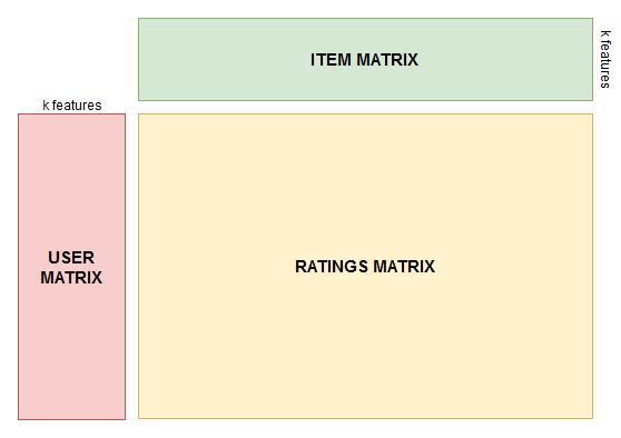
Rating Matrix | Recommender System
The rating matrix – obtained by the dot product of both user and item matrices. The features present in these matrices -known as Latent features and they act as constraints. These constraints are dependent on user preferences such as genres, the cast of the movie, director preference etc.
Let’s take a subset of the example and assume only two features, to better understand the process. For the user E:
It appears this user prefers movies related to space/sci-fi and superheroes, and as such tends to leave better ratings for such movies. Hence weightage for movies with these features is higher than for the others (given by 3 and 2 resp. in the diagram below).
Note: Here space-movie is used as a blanket term that refers to space, aliens, planets etc.
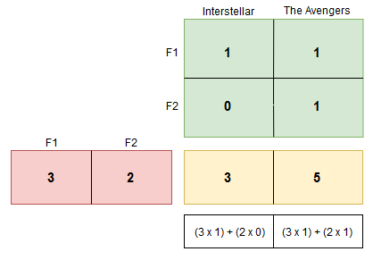
(Item Matrix: F1 – Space movie, F2 – Superheroes.)
Interstellar confirms the constraint of being a space related movie but fails to satisfy the superhero constraint. The avengers on the other hand, confirms to both constraints and as such the dot product of the matrices results in the highest ratings – i.e. 5.
Similarly, each of the other users have some preferences which the algorithm learns over time. The preferences are used as constraints in creating the user and item matrices. This method, although functionally similar to the previous ones, performs very well even when the matrix is sparsely populated.
As with any machine learning model, we must incorporate a cost function into this algorithm in order to optimize the factorisation process.
RMSE
Root Mean Squared Error or RMSE, is commonly used as the cost function.
1. The utility matrix is factorised.
2. The squared error for each available movie rating is calculated and the root of the mean of all the squared errors is calculated.
3. This root value is minimised using Gradient Descent or Altering Least Squares method.
4. The steps are repeated till an optimal solution is reached.
5. After the optimal factors are attained, we calculate the dot product with respect to the constraints to predict ratings for movies that haven’t been watched yet – i.e. the missing cell values in the sparse matrix.
The user is now provided with recommendations, and watching movies will no longer seem like a daunting task.
Conclusion:
There are many more processes and sub-processes that can be used to provide recommendations, but these are the commonly used tactics and are also relatively simple to grasp. This post only contains a fraction of the mathematics and logic behind recommender systems, but it is hoped that the content provides an engaging introduction to the field.
Although we only explored movie recommendation systems, the same principles apply to any scenario that requires this function. These systems are so common, especially in the e-commerce and food industry, that it would be nearly impossible not to come across them. Technology companies have greatly profited off of such an elegant concept, and it surely makes our lives as consumers far less cumbersome.
Article By: Shivaadith Anbarasu